Abstract
We introduce and study a minimal 1D model for the simulation of dynamic friction and dissipation at the atomic scale. This model consists of a point mass (slider) that moves over and interacts weakly with a linear chain of particles interconnected by springs, representing a crystalline substrate. This interaction converts a part of the kinetic energy of the slider into phonon waves in the substrate. As a result, the slider experiences a friction force. As a function of the slider speed, we observe dissipation peaks at specific values of the slider speed, whose nature we understand by means of a Fourier analysis of the excited phonon modes. By relating the phonon phase velocities with the slider velocity, we obtain an equation whose solutions predict which phonons are being excited by the slider moving at a given speed.
Introduction
Friction affects a wide variety of phenomena spanning broad ranges of length and time scales. Due to its practical and technological relevance, the study of friction was addressed even long before physics became a science. Fundamental steps in understanding its microscopic nature were achieved in the early 20th century [1-5]. Since the last decades of that century, major advancements in capturing the intimate relations between the atomistic dynamics and the dissipation mechanisms came as the result of the development of the atomic force microscope (AFM) and its friction force microscope (FFM) variant [6-8], as well as the extensive usage of atomistic molecular dynamics (MD) simulations and modeling made possible by the vastly increased computing power availability [9-16].
Despite this substantial progress, several fundamental mechanisms of friction and dissipation still need clarification. In particular, nanofriction (the study of friction at the atomic scale) lacks a theoretical model capable of accounting quantitatively for the dissipation of energy, i.e., the transformation of the kinetic energy of a macroscopic ordered motion into the internal energy of disordered thermal phonons. Both standard basic models of nanotribology, namely the Prandtl–Tomlinson model [1,2,13] and the Frenkel–Kontorova model [13,15-18], implement dissipation through a phenomenological viscous damping term acting on the physical degrees of freedom of the model. Moreover, such damping terms, beside affecting the dynamics, are characterized by a damping rate γ whose value is left to the arbitrary choice of the researcher. Finite-temperature is often simulated in the standard Langevin scheme, where to the viscous term one adds suitable Gaussian-distributed random forces, whose amplitude, via the fluctuation–dissipation theorem, is also affected by the value of γ [19].
A few approaches try to get rid of the arbitrariness of damping terms, describing dissipation explicitly. Microcanonical conservative simulations, for example, can describe the energy transfer into internal vibrational energy omitting all unphysical damping terms altogether [20-25]. The disadvantage of this approach is that, due to the finite and relatively small number of degrees of freedom available in a practical MD simulation cell, the dissipated energy accumulates in the phonons in the simulated sample, leading to a progressive overheating. Therefore this simulation procedure cannot address a steady sliding regime, but can at most identify the leading instabilities occurring and the most strongly coupled internal modes of the system. Another kind of approach involves using microcanonical equations to simulate a relatively broad cell including and surrounding the sliding contact region, adding dissipation through a suitable thermostat affecting only the atoms at the outer boundary of this region [26-35]. The main difficulty here is to provide a satisfactory implementation of the thermostat that not only provides a correct canonical dynamics in equilibrium conditions, but also manages to dispose of the extra excitation energy carried by the traveling phonon waves generated at the sliding contact, with minimal reflections at the boundary interface between conservative and thermostated particles. Such an implementation is in the process of being achieved [36-38], although with a rather intricate formalism, and should eventually become the technique of choice when one attempts to predict the sliding properties of a given physical interface for which a reliable force field is available. A third approach involves an uniformly distributed viscous damping term acting however only on the degrees of freedom perpendicular to the sliding direction [10,39,40]. While this method is quite effective in the context of fluid boundary lubrication, in the context of dry friction and crystalline interfaces nontrivial couplings of longitudinal and transverse modes [32,41,42] may lead to undesired γ-dependent effects.
In the present work we propose a different, minimalist approach, very much in the spirit of the Prandtl–Tomlinson and Frenkel–Kontorova (FK) models. We introduce and characterize a minimal slider–substrate model that captures the microscopic essentials of sliding friction and dissipation mechanisms, without the need of introducing ad hoc uncontrolled dissipative terms. This model consists only of a point-like localized cursor representing, e.g., a sharp AFM tip, interacting with an atomistic elastic substrate. As the slider skates on the elastically deformable crystal, phonons are generated and propagate away from the point of interaction. In this way, the slider mechanical energy is converted into crystal vibrational energy without any artificial viscous damping term affecting the slider itself. Of course, without any mechanism for dissipating this vibrational energy, the elastic substrate would eventually heat up as discussed above. For this reason we do include a weak viscous damping term, but this term acts on the elastic substrate only. We make sure that the effect of this term is negligible for the target of this research: the energy transfer from the slider to the substrate. This model virtually allows us to dispose of the arbitrary viscous damping, and to study the intrinsic dissipation properties of a sliding interface, as a function of several physical quantities, the most interesting of which is the sliding speed. Earlier work also investigated the speed dependence of the kinetic friction force in several models [1,25,43-50]. Under suitable conditions, specific velocities emerged as characterized by large kinetic friction due to suitable resonant conditions, in particular when the washboard frequency matches some phonon modes of the harmonic chain in the FK model [25,43]. In the present model too, characteristic resonances emerge at special speeds, but the resulting resonances differ significantly from those found for the FK model which represents an extended (infinite) solid–solid interface excited at a single wavelength, that of the sinusoidal potential. The present model focuses rather on the excitations induced by a localized point-like contact, inspired by an AFM tip, which has therefore the potentiality to generate excitations at all wavelengths.
This paper is organized as follows. Section “The Model” introduces our model. In Section “The kinetic friction force” we evaluate the kinetic friction as a function of the slider velocity. On top of a generally decreasing friction with sliding velocity, we identify peculiar “resonant” friction peaks at specific sliding velocities; in particular Subsection “Understanding: phonon phase velocities” draws a connection between the slider speed and the substrate phonon phase velocities, and proposes a relation that predicts the excited phonon modes when the slider advances at a given velocity, accounting for the observed dissipation peaks. In Section “Discussion and Conclusion” we discuss the obtained results, compare them to previous work, and sketch future extensions of the model. Appendix “The static friction force” reports and discusses the evaluation of the static friction threshold of this model.
The Model
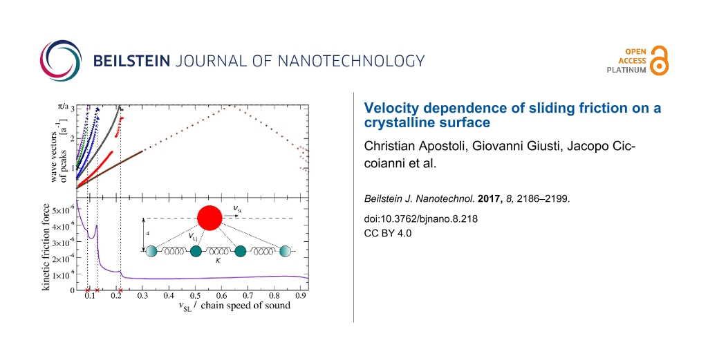
We propose the model sketched, in its simplest form, in Figure 1. It consists of a slider plus a linear chain of N point-like atoms. The chain atoms, of mass m and positions xj, are connected by harmonic springs to their nearest neighbors. The total harmonic potential is
![[2190-4286-8-218-i1]](/bjnano/content/inline/2190-4286-8-218-i1.svg?max-width=590&scale=1.18182)
where K is the elastic constant of the springs and a is the equilibrium lattice spacing. The simulation is carried out inside a periodically repeated supercell of size L = Na, so that, e.g., in Equation 1 xN+1 ≡ x1.
![[2190-4286-8-218-1]](/bjnano/content/figures/2190-4286-8-218-1.png?scale=2.0&max-width=1024&background=FFFFFF)
Figure 1: A sketch of the 1D slider-substrate model. The large sphere represents the slider, which moves along a fixed line (dashed) and interacts via Lennard–Jones forces with all atoms in the harmonic chain (smaller spheres).
Figure 1: A sketch of the 1D slider-substrate model. The large sphere represents the slider, which moves alon...
The slider is also a pointlike particle, with horizontal position xSL and mass mSL. We usually take mSL > m, but this condition is by no means required. The slider follows a guide at a fixed distance d from the chain and interacts with each chain atom through a Lennard–Jones (LJ) term. Indicating with Rj = [d2 + (xSL − xj)2]1/2 the distance between the slider and the j-th particle, the total slider-chain interaction energy is
![[2190-4286-8-218-i2]](/bjnano/content/inline/2190-4286-8-218-i2.svg?max-width=590&scale=1.18182)
where VLJ is the LJ potential
![[2190-4286-8-218-i3]](/bjnano/content/inline/2190-4286-8-218-i3.svg?max-width=590&scale=1.18182)
with equilibrium distance σ. The total potential energy Vharm + VSL−C combined with the appropriate kinetic terms governs the model dynamics, which can be either classic or quantum. In Section “Discussion and Conclusion” we will discuss a few straightforward generalizations of this model, namely the removal of the constraint of a fixed slider–chain distance; a structured slider consisting of many atoms; the chain replaced by a 2D or, more realistically, 3D crystal.
A sinusoidal wave propagating in the chain follows the textbook dispersion relation [51] between its angular frequency ω and its 1D wave vector k:
![[2190-4286-8-218-i4]](/bjnano/content/inline/2190-4286-8-218-i4.svg?max-width=590&scale=1.18182)
The corresponding long-wavelength speed of sound is
![[2190-4286-8-218-i5]](/bjnano/content/inline/2190-4286-8-218-i5.svg?max-width=590&scale=1.18182)
As discussed in the Introduction, the chain atoms are also affected by a weak viscous force, so that the phonon waves that propagate in the crystal get dampened and eventually fade while they move away from the point where they were generated, namely in the vicinity of the slider. The viscous force that acts on the j-th atom of the chain is
![[2190-4286-8-218-i6]](/bjnano/content/inline/2190-4286-8-218-i6.svg?max-width=590&scale=1.18182)
where γ is the damping coefficient. Thanks to this term, the oscillations generated by the slider are confined in a region smaller than the supercell, thus preventing the waves from coming back to the slider position.
In the present model all mechanical quantities can be expressed naturally in terms of the quantities a, m, and K characterizing the linear chain. Table 1 lists the natural units for the various mechanical quantities studied in the present work. For example, velocity is measured in units of the chain speed of sound vs: this means that, e.g., a slider speed |vSL| exceeding unity is a supersonic speed.
In most simulations, unless otherwise specified, we adopt the following standard set of parameters: L = 500a, i.e., a chain formed by N = 500 atoms; a weak slider–chain coupling ε = 5 × 10⁻⁴ Ka2; slider mass mSL = 10m; and chain damping γ = 0.1 (mK)1/2. We take a rather small LJ radius σ = 0.5a, and adopt an even closer approach distance between the slider and the chain d = 0.475a. The effect of this d < σ choice is to generate a periodic double-minimum effective potential experienced by the advancing slider in the limit where one could neglect the displacements of chain atoms, see the solid line of Figure 2. In contrast, a larger d > σ would rather produce a potential of the type depicted by the dashed line of Figure 2: for simplicity, we defer the investigation of the d > σ scenario to future work.
![[2190-4286-8-218-2]](/bjnano/content/figures/2190-4286-8-218-2.png?scale=2.0&max-width=1024&background=FFFFFF)
Figure 2: The potential-energy profile experienced by the slider as it moves along a hypothetical chain with atoms frozen at positions xj = ja (big circles), for a LJ parameter σ = 0.5a. Dashed curve: as obtained with d = 0.525a > σ; solid curve: with d = 0.475a < σ, the value adopted for the rest of this work.
Figure 2: The potential-energy profile experienced by the slider as it moves along a hypothetical chain with ...
The Kinetic Friction Force
Simulation protocols
To evaluate a meaningful estimate of the kinetic, or dynamic, friction force experienced by the advancing slider, we develop two alternative protocols [52,53]. In protocol A we first execute a “run-in” calculation at constant speed vSL, that allows the initial shock waves induced by the sudden apparition of the slider near the chain to die out. Starting from the dynamical condition reached at the end of the first simulation, we then run a second simulation in which the slider is allowed to change its velocity as a consequence of the interaction with the chain and its own inertia like, e.g., in “ballistic” experiments where clusters deposited at surfaces are kicked around until they come to rest dissipating their kinetic energy into the substrate [49,54-56]. Figure 3 displays an example of the time dependence obtained in such second simulation. From the slider mean slowing rate during this second simulation, one can extract the kinetic friction force with the following method: time is divided into regular intervals, e.g., of 5000 time units, a very long time compared to the period of the fluctuations of vSL; then a linear regression is performed over each interval; the (negative) slope of the straight line fitting vSL as a function of time represents the slider average acceleration. The average dynamic friction force Fd experienced by the slider is then obtained by multiplying this acceleration by (−mSL). Associating this value of Fd to the mean value of vSL in the same time interval, one obtains the dependence Fd(vSL). The faster and faster slider slowing rate displayed in Figure 3a indicates an increasing dynamic friction Fd(vSL) as its speed vSL decreases. As vSL decreases and friction increases, the chain center-of-mass velocity vCM oscillates more and more, a useful indicator of a larger and larger transfer of momentum from the slider to the chain. Of course the observed small-amplitude oscillations of vCM are almost entirely the result of the oscillations induced in the few chain atoms directly interacting with the slider, with the vast majority of far-away atoms remaining essentially stationary. These center-of-mass oscillations are therefore an artifact of the finite size of the chain, and would vanish entirely in the macroscopic-size limit.
![[2190-4286-8-218-3]](/bjnano/content/figures/2190-4286-8-218-3.png?scale=2.0&max-width=1024&background=FFFFFF)
Figure 3: The time dependence (a) and (b) of the slider velocity vSL and (c) of the chain center of mass vCM for the second simulation (freely-slowing mode) of protocol A. The simulation is carried out until the slider finally stops and dissipates its residual energy in oscillations expanded in the inset (b), around a minimum of the effective potential of Figure 2, with chain phonon waves carrying this residual energy away, until the eventual complete arrest of the system. Note the increasing negative mean slope of the vSL curve, indicating an increasing mean friction force Fd as vSL decreases.
Figure 3: The time dependence (a) and (b) of the slider velocity vSL and (c) of the chain center of mass vCM ...
Protocol B is as follows: we execute a single calculation keeping vSL constant, as if the slider was an AFM tip attached to an infinitely rigid AFM cantilever, wait until a steady-sliding regime is established, and discard the initial part affected by transients. For the remaining part of the simulation, we record the total force experienced by the slider as a function of time. This force has fluctuations as a result of collisions against the consecutive atoms of the chain. The period of these fluctuations is a/vSL. We average this force over an integer number of these periods, and interpret the result as the average friction force Fd corresponding to the velocity vSL. We start over a new simulation for every value of vSL of interest.
While protocol A evaluates rigorously the friction force, allowing for all kinds of acceleration–deceleration effects related to individual slider–atom collisions, protocol B would coincide with protocol A only in the limit where the energy transferred in a single atomic collision is much smaller than the kinetic energy accumulated in the slider. The LJ parameter ε provides a conservative estimate of the energy transferred in the collision: the condition for a rigorous applicability of protocol B is
![[2190-4286-8-218-i7]](/bjnano/content/inline/2190-4286-8-218-i7.svg?max-width=590&scale=1.18182)
This means that protocol B should yield results identical to protocol A for vSL ≥ (2 ε/mSL)1/2 ![[Graphic 1]](/bjnano/content/inline/2190-4286-8-218-i20.svg?max-width=637&scale=1.18182) 10−2 vs for the standard simulation parameters introduced above. We have verified numerically that this is indeed the case. We have also verified numerically that in the considered weak-coupling regime, Fd
10−2 vs for the standard simulation parameters introduced above. We have verified numerically that this is indeed the case. We have also verified numerically that in the considered weak-coupling regime, Fd ![[Graphic 2]](/bjnano/content/inline/2190-4286-8-218-i21.svg?max-width=637&scale=1.18182) ε2. This is in accord with the observation that the dissipated power FdvSL must equal the average work per unit time done by the slider on the chain. The latter equals the product of the force exerted by the slider on each chain atom times that atom’s velocity vj. The force is of course proportional to the coupling ε and, to first order in ε/(Ka2), also vj is proportional to ε, whence the Fd
ε2. This is in accord with the observation that the dissipated power FdvSL must equal the average work per unit time done by the slider on the chain. The latter equals the product of the force exerted by the slider on each chain atom times that atom’s velocity vj. The force is of course proportional to the coupling ε and, to first order in ε/(Ka2), also vj is proportional to ε, whence the Fd ![[Graphic 3]](/bjnano/content/inline/2190-4286-8-218-i22.svg?max-width=637&scale=1.18182) ε2 dependence at weak coupling.
ε2 dependence at weak coupling.
Incidentally note that, in both protocols, the slider transfers not only energy but also momentum to the chain. Indeed the friction force Fd equals precisely the transfer of momentum per unit time from the slider to the chain. Fd is negative (leftward) when considered acting on the slider; due to the Newton’s third law, the chain experiences a positive (rightward) force of precisely the same intensity. As a combined result of Fd and the damping force provided by the dissipative terms of Equation 6, in the steady regime the slider acquires a small but nonzero mean center-of-mass velocity vCM. As a result, the slider speed relative to the chain is decreased relative to the imposed vSL,abs, precisely by ![[Graphic 4]](/bjnano/content/inline/2190-4286-8-218-i23.svg?max-width=637&scale=1.18182) In the following, we denote by vSL,abs the slider velocity in the lab frame, and by vSL the slider velocity in the frame of the chain center of mass:
In the following, we denote by vSL,abs the slider velocity in the lab frame, and by vSL the slider velocity in the frame of the chain center of mass:
![[2190-4286-8-218-i8]](/bjnano/content/inline/2190-4286-8-218-i8.svg?max-width=590&scale=1.18182)
In practice, we obtain vCM /vSL,abs ![[Graphic 5]](/bjnano/content/inline/2190-4286-8-218-i24.svg?max-width=637&scale=1.18182) 1 for not-too-small vSL,abs, so that this correction is irrelevant, and vSL
1 for not-too-small vSL,abs, so that this correction is irrelevant, and vSL ![[Graphic 6]](/bjnano/content/inline/2190-4286-8-218-i25.svg?max-width=637&scale=1.18182) vSL,abs. However at low speed this correction can become significant.
vSL,abs. However at low speed this correction can become significant.
Control of the dissipation terms
First off, we need to identify a range for the dissipation parameter γ where the dissipative terms of Equation 6 become irrelevant to the frictional dynamics. Figure 4 displays the dependence of the sliding friction measured for vSL = 0.1 vs, obtained repeating the simulations with different values of the damping parameter γ. This figure shows that for large and increasing γ, friction tends to decrease. This is expected, since in the unphysical strongly overdamped regime, it is harder and harder to displace the chain atoms away from their equilibrium positions, with the result that their effect on the slider resembles more and more closely that of a conservative effective potential, namely the one of Figure 2, which of course allows for no energy transfer, and no dissipation. As damping is decreased to the physically relevant underdamped region γ < (mK)1/2, friction stabilizes to a physically significant γ-independent value. However, when γ is further decreased below approximately 10−2 (mK)1/2, the waves produced at the slider–chain contact point become less and less damped, see Figure 5. When the γ value becomes too small, the phonon waves propagate all the way across the periodically repeated cell, eventually returning to the slider–chain contact point. As a result, the chain slides over an effectively “hot” substrate, generating an unphysical friction reduction related to thermolubricity [45,46,57-62]. As shown by the circles in Figure 4, a much longer chain provides enough space for the phonon waves to decay, thus allowing the phonon amplitude to be radically reduced before returning to slider-chain contact point, even with small γ. In the following we adopt γ = 0.1(mK)1/2 as the standard value of the damping rate, unless otherwise indicated.
![[2190-4286-8-218-4]](/bjnano/content/figures/2190-4286-8-218-4.png?scale=2.0&max-width=1024&background=FFFFFF)
Figure 4: The dynamical friction force as a function of the damping coefficient γ that fixes the (unphysical) dissipation rate of the chain atoms. This is evaluated for vSL = 0.1 vs with protocol A (but protocol B provides identical data). Squares: simulations executed in a standard supercell of size L = 500a, with 500 atoms. Circles: similar simulations executed in a 10× longer supercell with 5000 atoms, where the waves emitted by the slider have a much longer space to decay fully before coming back to the contact point, even for smaller γ.
Figure 4: The dynamical friction force as a function of the damping coefficient γ that fixes the (unphysical)...
![[2190-4286-8-218-5]](/bjnano/content/figures/2190-4286-8-218-5.png?scale=2.0&max-width=1024&background=FFFFFF)
Figure 5: Three snapshots of the instantaneous velocities of a few chain atoms as a function of their position while interacting with the slider, whose instantaneous position xSL is marked by a vertical dashed line. The three calculations are executed with the same vSL = 0.1 vs, but with three different values of γ, which produce visibly different damping of the same excited phonon waves away from the interaction point.
Figure 5: Three snapshots of the instantaneous velocities of a few chain atoms as a function of their positio...
Sliding-speed dependence of friction
Figure 6 shows the speed dependence of the kinetic friction Fd. The general trend is of a decreasing friction with speed. In particular, Fd drops dramatically to 0 when vSL exceeds the speed of sound of the chain. In the region below the speed of sound (vertical dotted line) Fd stands on a relatively stable plateau. Several friction peaks then emerge in the region roughly between 10% and 20% vs. When vSL is further decreased, friction starts to rise approximately as ![[Graphic 7]](/bjnano/content/inline/2190-4286-8-218-i26.svg?max-width=637&scale=1.18182) (where A is a constant), although, with the standard parameters of Section “The Model”, a deviation is observed quite early, for vSL
(where A is a constant), although, with the standard parameters of Section “The Model”, a deviation is observed quite early, for vSL ![[Graphic 8]](/bjnano/content/inline/2190-4286-8-218-i27.svg?max-width=637&scale=1.18182) 0.03 vs. This deviation is not particularly related to reaching the speed region where protocol B, introduced in Section “Simulation protocols” above, becomes unreliable. We have verified that this deviation is instead an artifact of the damping in the chain. By repeating the simulations with a longer chain (L = 105a) and smaller damping γ = 10−4(mK)1/2, we find that the Fd =
0.03 vs. This deviation is not particularly related to reaching the speed region where protocol B, introduced in Section “Simulation protocols” above, becomes unreliable. We have verified that this deviation is instead an artifact of the damping in the chain. By repeating the simulations with a longer chain (L = 105a) and smaller damping γ = 10−4(mK)1/2, we find that the Fd = ![[Graphic 9]](/bjnano/content/inline/2190-4286-8-218-i28.svg?max-width=637&scale=1.18182) regime persists down to vSL
regime persists down to vSL ![[Graphic 10]](/bjnano/content/inline/2190-4286-8-218-i29.svg?max-width=637&scale=1.18182) 10−3 vs. With the adopted value for the coupling ε, protocol A cannot determine friction reliably as a function of vSL in this region of speeds, because vSL itself oscillates widely in time as the slider nears stopping, see Figure 3b. However we reduced the coupling ε by one order of magnitude to ε = 5 × 10⁻⁵ Ka2, and verified that the points of the N = 105, γ = 10−4 (mK)1/2 curve are perfectly reproducible, apart from a factor 10−2 smaller friction, thus confirming the Fd =
10−3 vs. With the adopted value for the coupling ε, protocol A cannot determine friction reliably as a function of vSL in this region of speeds, because vSL itself oscillates widely in time as the slider nears stopping, see Figure 3b. However we reduced the coupling ε by one order of magnitude to ε = 5 × 10⁻⁵ Ka2, and verified that the points of the N = 105, γ = 10−4 (mK)1/2 curve are perfectly reproducible, apart from a factor 10−2 smaller friction, thus confirming the Fd = ![[Graphic 11]](/bjnano/content/inline/2190-4286-8-218-i30.svg?max-width=637&scale=1.18182) low-speed scaling.
low-speed scaling.
![[2190-4286-8-218-6]](/bjnano/content/figures/2190-4286-8-218-6.png?scale=2.0&max-width=1024&background=FFFFFF)
Figure 6: Dynamic friction force as a function of the slider speed vSL. For comparison, the horizontal dashed line marks the static-friction threshold Fstatic obtained in Appendix “The static friction force”, Equation 16. The vertical dotted line marks the speed of sound vs. The data are obtained by means of protocol B; we verified that perfectly superposable curves can be obtained by means of protocol A as long as it can be effectively applied, i.e., as long as the friction force Fd < 10−5 Ka.
Figure 6: Dynamic friction force as a function of the slider speed vSL. For comparison, the horizontal dashed...
As shown in Figure 3, the simulations of this model do provide concrete realizations of the dynamic to static transition. Unfortunately, due to the wide oscillations displayed in Figure 3b, the transition from dynamic to static friction is just impossible to characterize in terms of a simple function Fd(vSL). We evaluate the static friction for this model as detailed in Appendix “The static friction force”. The comparison of Fd and Fstatic in Figure 6 confirms that of course this model is consistent with the well-known result that Fd < Fstatic.
We should now investigate the reason for the friction peaks at certain special subsonic velocities. For this purpose, we must identify what phonon modes are most strongly excited at each particular slider speed.
Phonon excitations
The friction force Fd of Figure 6 dissipates the slider kinetic energy by transforming it into phonon waves that travel away from the contact point, as illustrated in Figure 5. We analyze these phonon excitations for several values of vSL. We must first detail the protocol of this analysis.
We run a simulation with fixed slider speed vSL,abs. At a given time t after the end of the initial transient, we take a snapshot of the individual velocities vj of the chain atoms, as in the example of Figure 7a. We then execute a spatial Fourier transform of these instantaneous velocities:
![[2190-4286-8-218-i9]](/bjnano/content/inline/2190-4286-8-218-i9.svg?max-width=590&scale=1.18182)
Here i is the imaginary unit and k spans the first Brillouin zone (BZ) (−π/a, π/a]. Figure 7b displays ![[Graphic 12]](/bjnano/content/inline/2190-4286-8-218-i31.svg?max-width=637&scale=1.18182) for the velocity pattern of Figure 7a. Observe first that the real values of vj guarantee that
for the velocity pattern of Figure 7a. Observe first that the real values of vj guarantee that ![[Graphic 13]](/bjnano/content/inline/2190-4286-8-218-i32.svg?max-width=637&scale=1.18182) and therefore that
and therefore that ![[Graphic 14]](/bjnano/content/inline/2190-4286-8-218-i33.svg?max-width=637&scale=1.18182) is an even function of k, as is evident in Figure 7b. Due to this symmetry in all following figures reporting Fourier transforms we will display the positive half [0, π/a] of the first BZ only.
is an even function of k, as is evident in Figure 7b. Due to this symmetry in all following figures reporting Fourier transforms we will display the positive half [0, π/a] of the first BZ only.
![[2190-4286-8-218-7]](/bjnano/content/figures/2190-4286-8-218-7.png?scale=2.0&max-width=1024&background=FFFFFF)
Figure 7:
(a): A snapshot of the velocities of the chain particles while the slider, instantly at the vertical dashed-line position, advances at vSL = 0.1 vs. (b): The square modulus of the spatial Fourier transform ![[Graphic 15]](/bjnano/content/inline/2190-4286-8-218-i34.svg?max-width=637&scale=1.18182) (k, t) of the velocities, as defined in Equation 9.
(k, t) of the velocities, as defined in Equation 9.
Figure 7: (a): A snapshot of the velocities of the chain particles while the slider, instantly at the vertica...
The peaks of the Fourier transform highlight the phonons most excited by the interaction with the slider at that given instant in time. For a given vSL, during the simulation the velocity pattern vj(t), and therefore its Fourier transform, evolve in time. We take advantage of the fact that the slider encounters the chain particles at a regular interval T = a/vSL: in the steady state vj(t) is a periodic function of time but for a lattice translation, vj+1(t + T) = vj(t). As a global translation (a shift in j) only affects the phase of ![[Graphic 16]](/bjnano/content/inline/2190-4286-8-218-i35.svg?max-width=637&scale=1.18182) (k, t), but not its amplitude,
(k, t), but not its amplitude, ![[Graphic 17]](/bjnano/content/inline/2190-4286-8-218-i36.svg?max-width=637&scale=1.18182) is exactly periodic in time:
is exactly periodic in time:
![[2190-4286-8-218-i10]](/bjnano/content/inline/2190-4286-8-218-i10.svg?max-width=590&scale=1.18182)
Figure 8 displays an example of this periodic time dependence of ![[Graphic 18]](/bjnano/content/inline/2190-4286-8-218-i37.svg?max-width=637&scale=1.18182) .
.
![[2190-4286-8-218-8]](/bjnano/content/figures/2190-4286-8-218-8.png?scale=2.0&max-width=1024&background=FFFFFF)
Figure 8:
The square modulus of the Fourier transforms of the velocities vj(t), at six subsequent times. Here the slider velocity is vSL = 0.1 vs. Comparing the plots of ![[Graphic 19]](/bjnano/content/inline/2190-4286-8-218-i38.svg?max-width=637&scale=1.18182) and
and ![[Graphic 20]](/bjnano/content/inline/2190-4286-8-218-i39.svg?max-width=637&scale=1.18182) , one sees that
, one sees that ![[Graphic 21]](/bjnano/content/inline/2190-4286-8-218-i40.svg?max-width=637&scale=1.18182) repeats itself identically after one entire period T = a/vSL = 10 (m/K)1/2.
repeats itself identically after one entire period T = a/vSL = 10 (m/K)1/2.
Figure 8: The square modulus of the Fourier transforms of the velocities vj(t), at six subsequent times. Here...
To obtain a time-independent description of the typical phonon-excitation spectrum at a given vSL, we average the square modulus of ![[Graphic 22]](/bjnano/content/inline/2190-4286-8-218-i41.svg?max-width=637&scale=1.18182) over a period T. We select M = 50 instants of time, equally spaced within the period, and compute
over a period T. We select M = 50 instants of time, equally spaced within the period, and compute ![[Graphic 23]](/bjnano/content/inline/2190-4286-8-218-i42.svg?max-width=637&scale=1.18182) at each of them. Then we calculate the time-averaged Fourier transform as follows:
at each of them. Then we calculate the time-averaged Fourier transform as follows:
![[2190-4286-8-218-i11]](/bjnano/content/inline/2190-4286-8-218-i11.svg?max-width=590&scale=1.18182)
We verified that a finer sampling of the period (larger M) shows no significant difference in this average spectral intensity.
Figure 9 illustrates the resulting time-averaged power spectra ![[Graphic 24]](/bjnano/content/inline/2190-4286-8-218-i43.svg?max-width=637&scale=1.18182) for a few sample velocities vSL. Figure 9a shows that for supersonic vSL the power spectrum is quite flat, with no sharp peak: most phonon modes are excited with comparable, rather weak, intensities; only those closest to k = 0 are left substantially unexcited. When vSL is less than the speed of sound vs, but greater than
for a few sample velocities vSL. Figure 9a shows that for supersonic vSL the power spectrum is quite flat, with no sharp peak: most phonon modes are excited with comparable, rather weak, intensities; only those closest to k = 0 are left substantially unexcited. When vSL is less than the speed of sound vs, but greater than ![[Graphic 25]](/bjnano/content/inline/2190-4286-8-218-i44.svg?max-width=637&scale=1.18182) 0.217 vs, as in Figure 9b, the spectrum is dominated by a single peak. As vSL is lowered below
0.217 vs, as in Figure 9b, the spectrum is dominated by a single peak. As vSL is lowered below ![[Graphic 26]](/bjnano/content/inline/2190-4286-8-218-i45.svg?max-width=637&scale=1.18182) 0.217 vs, as in Figure 9c,d, multiple peaks appear, and, as vSL decreases, their number increases progressively. As vSL further decreases, Figure 9e, the positions of all peaks approach k = 0, where they gradually merge into a single peak, Figure 9f. Note that the spectral resolution is limited both by the finite chain length, with δk = 2π/(Na), see Equation 9, and by the phonon localization induced by the damping term of Equation 6.
0.217 vs, as in Figure 9c,d, multiple peaks appear, and, as vSL decreases, their number increases progressively. As vSL further decreases, Figure 9e, the positions of all peaks approach k = 0, where they gradually merge into a single peak, Figure 9f. Note that the spectral resolution is limited both by the finite chain length, with δk = 2π/(Na), see Equation 9, and by the phonon localization induced by the damping term of Equation 6.
![[2190-4286-8-218-9]](/bjnano/content/figures/2190-4286-8-218-9.png?scale=2.0&max-width=1024&background=FFFFFF)
Figure 9:
The time-averaged square modulus of the Fourier transform of the chain velocities, for a few characteristic values of vSL: (a) supersonic speed; (b) single-peak subsonic region; (c) appearance of the second pair of peaks; (d) multi peak region near vSL ![[Graphic 27]](/bjnano/content/inline/2190-4286-8-218-i46.svg?max-width=637&scale=1.18182) 0.1 vs; (e) small-speed collapse of the dissipation peaks toward k = 0; (f) full collapse to one peak at very small vSL
0.1 vs; (e) small-speed collapse of the dissipation peaks toward k = 0; (f) full collapse to one peak at very small vSL ![[Graphic 28]](/bjnano/content/inline/2190-4286-8-218-i47.svg?max-width=637&scale=1.18182) vs.
vs.
Figure 9: The time-averaged square modulus of the Fourier transform of the chain velocities, for a few charac...
Figure 10 tracks the positions and intensities of the observed peaks of ![[Graphic 29]](/bjnano/content/inline/2190-4286-8-218-i48.svg?max-width=637&scale=1.18182) as functions of vSL. These data are obtained by fitting the functions
as functions of vSL. These data are obtained by fitting the functions ![[Graphic 30]](/bjnano/content/inline/2190-4286-8-218-i49.svg?max-width=637&scale=1.18182) with sums of up to 7 Lorentzian curves. Figure 10 reports the centers and heights of the fitted Lorentzian terms.
with sums of up to 7 Lorentzian curves. Figure 10 reports the centers and heights of the fitted Lorentzian terms.
![[2190-4286-8-218-10]](/bjnano/content/figures/2190-4286-8-218-10.png?scale=2.0&max-width=1024&background=FFFFFF)
Figure 10:
The positions (a) and heights (b) of the peaks of ![[Graphic 31]](/bjnano/content/inline/2190-4286-8-218-i50.svg?max-width=637&scale=1.18182) as functions of vSL. Panels (c) and (d): detail of the vSL ≤ 0.23 vs low-speed region for the same quantities.
as functions of vSL. Panels (c) and (d): detail of the vSL ≤ 0.23 vs low-speed region for the same quantities.
Figure 10:
The positions (a) and heights (b) of the peaks of as functions of vSL. Panels (c) and (d): detail ...
Even in the supersonic region vSL > vs, where the phonon power spectrum is smooth and flat and lacks sharp peaks as in Figure 9a, we fit the spectrum with the sum of four Lorentzian curves. These four Lorentzian profiles do their best to interpolate that continuum spectrum. Not surprisingly, the Lorentzian centers and intensities, displayed at the right side of Figure 10, follow a rather erratic variation with vSL, confirming that in the spectrum for supersonic sliding no sharp peak is actually present.
As vSL decreases below approximately 90% of the speed of sound, initially a single prominent peak appears near the BZ boundary (Figure 9b), tracked in wave vector and intensity by the crosses in the central region of Figure 10a,b. As vSL decreases below 0.217 vs, more peaks appear near the BZ boundary too, as in the examples of Figure 9c,d, and tracked explicitly in Figure 10c,d. As vSL is further decreased all peaks move down toward k = 0 and eventually merge for vSL ![[Graphic 32]](/bjnano/content/inline/2190-4286-8-218-i51.svg?max-width=637&scale=1.18182) vs, due to the finite k-resolution (Figure 9e,f). Figure 10c clarifies a nontrivial feature of this velocity-dependent phonon spectrum: except for the single peak emerging at vSL
vs, due to the finite k-resolution (Figure 9e,f). Figure 10c clarifies a nontrivial feature of this velocity-dependent phonon spectrum: except for the single peak emerging at vSL ![[Graphic 33]](/bjnano/content/inline/2190-4286-8-218-i52.svg?max-width=637&scale=1.18182) vs, all other new peaks appear in pairs.
vs, all other new peaks appear in pairs.
Figure 11 highlights the relation between the appearance of new peaks in the chain phonon spectrum of excitations at certain speeds with jumps in the dynamic friction Fd as a function of vSL. The important conclusion of this correlation is the following: dissipation increases suddenly for those values of vSL where new phonon modes start to get excited.
![[2190-4286-8-218-11]](/bjnano/content/figures/2190-4286-8-218-11.png?scale=2.0&max-width=1024&background=FFFFFF)
Figure 11:
A direct comparison of the peak wave vectors of ![[Graphic 34]](/bjnano/content/inline/2190-4286-8-218-i53.svg?max-width=637&scale=1.18182) , with the dynamic friction Fd as a function of vSL over the interesting speed range of Figure 6. The dotted vertical lines highlight the relation of the peaks of Fd with the appearance of new pairs of excited phonons near the BZ boundary.
, with the dynamic friction Fd as a function of vSL over the interesting speed range of Figure 6. The dotted vertical lines highlight the relation of the peaks of Fd with the appearance of new pairs of excited phonons near the BZ boundary.
Figure 11:
A direct comparison of the peak wave vectors of , with the dynamic friction Fd as a function of vSL...
Understanding: phonon phase velocities
Given the simplicity of this 1D model and the special weak-coupling regime investigated, we should be able to understand why certain phonons get excited at certain special speeds. We formulate the hypothesis that phonon modes get excited when their phase velocities ω/|k| match the slider speed vSL. We start by searching all values of k such that the phonon phase velocity matches a given speed vSL:
![[2190-4286-8-218-i12]](/bjnano/content/inline/2190-4286-8-218-i12.svg?max-width=590&scale=1.18182)
We substitute the simple dispersion relation ω(k) of Equation 4, and reformulate Equation 12 as:
![[2190-4286-8-218-i13]](/bjnano/content/inline/2190-4286-8-218-i13.svg?max-width=590&scale=1.18182)
This equation is put in dimensionless form by introducing ![[Graphic 35]](/bjnano/content/inline/2190-4286-8-218-i54.svg?max-width=637&scale=1.18182) and the parameter
and the parameter ![[Graphic 36]](/bjnano/content/inline/2190-4286-8-218-i55.svg?max-width=637&scale=1.18182)
![[2190-4286-8-218-i14]](/bjnano/content/inline/2190-4286-8-218-i14.svg?max-width=590&scale=1.18182)
For a given V (or equivalently a given vSL), the solutions x (or equivalently k) of Equation 14 (or equivalently Equation 13) provide the special wave vectors such that the phonon phase velocity matches the given speed vSL.
Equation 14 can of course be solved numerically for any V. An example of graphic solution of Equation 13 is displayed in Figure 12a. The resulting wave vectors are scattered over several BZs. We then bring all the k-point solutions inside the first BZ, Figure 12b. Finally, we proceed to compare these solutions to the positions of the peaks of the power spectrum ![[Graphic 37]](/bjnano/content/inline/2190-4286-8-218-i56.svg?max-width=637&scale=1.18182) obtained by MD at that specific slider speed, Figure 12c. In the example of Figure 12, this procedure is followed for vSL = 0.12 vs, showing that the solutions of Equation 13 match perfectly the positions of all observed peaks in the spectrum. In particular, Figure 12a clarifies why, for decreasing vSL, new excited phonon modes always arise near, but not quite at, the BZ boundary.
obtained by MD at that specific slider speed, Figure 12c. In the example of Figure 12, this procedure is followed for vSL = 0.12 vs, showing that the solutions of Equation 13 match perfectly the positions of all observed peaks in the spectrum. In particular, Figure 12a clarifies why, for decreasing vSL, new excited phonon modes always arise near, but not quite at, the BZ boundary.
![[2190-4286-8-218-12]](/bjnano/content/figures/2190-4286-8-218-12.png?scale=2.0&max-width=1024&background=FFFFFF)
Figure 12: A scheme of the steps performed to identify the phonons whose phase velocity equals vSL, and the comparison of the obtained wave vectors with the observed excited phonons peaks for the same slider velocity vSL. In this example vSL = 0.12 vs.
Figure 12: A scheme of the steps performed to identify the phonons whose phase velocity equals vSL, and the co...
Figure 13 compares the positions of the peaks of ![[Graphic 38]](/bjnano/content/inline/2190-4286-8-218-i57.svg?max-width=637&scale=1.18182) obtained from the analysis of MD trajectories as in Figure 10, with the wave vectors of the phonons whose phase velocity equals vSL, obtained by solving Equation 13. It is apparent that for vSL
obtained from the analysis of MD trajectories as in Figure 10, with the wave vectors of the phonons whose phase velocity equals vSL, obtained by solving Equation 13. It is apparent that for vSL ![[Graphic 39]](/bjnano/content/inline/2190-4286-8-218-i58.svg?max-width=637&scale=1.18182) 0.9 vs the two quantities match almost perfectly. We conclude that Equation 13 provides a reliable prediction of the wave vectors of the excited phonons for a given vSL. Above the speed of sound vs, Equation 13 has no solution and indeed the spectrum displays no sharp peak, see Figure 9a. Correspondingly the “nonresonant” friction is very small, see the right side of Figure 6.
0.9 vs the two quantities match almost perfectly. We conclude that Equation 13 provides a reliable prediction of the wave vectors of the excited phonons for a given vSL. Above the speed of sound vs, Equation 13 has no solution and indeed the spectrum displays no sharp peak, see Figure 9a. Correspondingly the “nonresonant” friction is very small, see the right side of Figure 6.
![[2190-4286-8-218-13]](/bjnano/content/figures/2190-4286-8-218-13.png?scale=2.0&max-width=1024&background=FFFFFF)
Figure 13:
The positions of the observed peaks of ![[Graphic 40]](/bjnano/content/inline/2190-4286-8-218-i59.svg?max-width=637&scale=1.18182) (symbols), compared with the values of k of the phonons whose phase velocity is equal to vSL (black solid lines), solutions of Equation 13. Inset: a blow up of the interval 0 ≤ vSL ≤ 0.23 vs.
(symbols), compared with the values of k of the phonons whose phase velocity is equal to vSL (black solid lines), solutions of Equation 13. Inset: a blow up of the interval 0 ≤ vSL ≤ 0.23 vs.
Figure 13:
The positions of the observed peaks of (symbols), compared with the values of k of the phonons who...
In particular Equation 13 allows us to predict the number and wave vectors of the excited phonon modes when the slider is moving at a given velocity. The number Nph of excited phonon modes at a given vSL is null for any vSL > vs, it turns to unity for 0.217 vs < vSL < vs, and then for smaller and smaller vSL Nph increases by two every time the dashed line of Figure 12a crosses one more sine hump. As a result, in the limit of small vSL, Nph is approximately
![[2190-4286-8-218-i15]](/bjnano/content/inline/2190-4286-8-218-i15.svg?max-width=590&scale=1.18182)
We have then a number of excited phonons which is inversely proportional to vSL for small vSL. The comparison of Figure 11 suggests that an increasing number of excited phonon modes leads to an increasing kinetic friction Fd, see Figure 11. If a comparable power was dissipated in each of the excited phonon modes, then Equation 15 would be compatible with the power-law dependence Fd(vSL) ![[Graphic 41]](/bjnano/content/inline/2190-4286-8-218-i60.svg?max-width=637&scale=1.18182) A/vSL that we observe in the low-speed regime in Figure 6. However there is no evidence that the same power is dissipated in each one of the phonon modes. In fact, Figure 10b,d shows that different modes draw different spectral weights. A systematic study of the intensities of the phonon excitations would probably be useful in understanding the Fd(vSL)
A/vSL that we observe in the low-speed regime in Figure 6. However there is no evidence that the same power is dissipated in each one of the phonon modes. In fact, Figure 10b,d shows that different modes draw different spectral weights. A systematic study of the intensities of the phonon excitations would probably be useful in understanding the Fd(vSL) ![[Graphic 42]](/bjnano/content/inline/2190-4286-8-218-i61.svg?max-width=637&scale=1.18182) A/vSL behavior in detail.
A/vSL behavior in detail.
Discussion and Conclusion
We introduce a new model, or rather a model class, that allows one to investigate friction at the very point where it is generated: the contact point. In the present paper we examine the main predictions of this model in its most basic incarnation: a point-like slider kept at a fixed distance to a 1D harmonic chain of masses and springs. The main result is that kinetic friction should depend on speed as a generally decreasing function, with several nontrivial features deviating from monotonicity: friction peaks arise every time a new “resonance condition” is fulfilled, namely that the phase velocity of some substrate phonon mode matches the slider speed. Recently published research also identified relations between dissipation peaks and the properties of a dispersion relation in a different model [63].
The present model can also be investigated in a spring-pulling scheme analogous to the Prandtl–Tomlinson model, to simulate the finite stiffness of an AFM cantilever. In that scheme a stick-slip to smooth-sliding transition can also be investigated, especially at low speed (see Appendix “The static friction force”), allowing one to study in detail the nonlinear phenomena and mechanisms of phonon excitations that arise at slip times. The stick-slip regime and the associated nonlinear phenomena will of course be more significant when the model is studied in a realistic regime of intermediate to strong coupling ε ≈ Ka2. We defer this investigation to future work, which should provide a microscopic basis and the limits of applicability for the Prandtl–Tomlinson model. This simple 1D model, studied in the spirit of protocol B (fixed slider speed) for weak slider-chain coupling ε ![[Graphic 43]](/bjnano/content/inline/2190-4286-8-218-i62.svg?max-width=637&scale=1.18182) Ka2, should be suitable to address even by means of analytic perturbative many-body methods. We plan to pursue this investigation in the future.
Ka2, should be suitable to address even by means of analytic perturbative many-body methods. We plan to pursue this investigation in the future.
The FK model and the present model both describe dissipation in terms of the excitations of the phonon modes of a linear harmonic chain. Therefore, the two models agree that no resonant energy transfer can occur for very large speed, and friction drops to 0, as at the right side of Figure 6. However, the frictional features demonstrated in the present work differ significantly from those found for the superlubric weak-corrugation regime of the FK model [25,43]. Specifically, in the FK model the condition for dissipation peaks, where center-mass translational energy is converted rapidly into internal phononic degrees of freedom, requires that the modulation dictated by the chain-potential lattice incommensurability resonates with the washboard frequency at the center-mass sliding velocity, due to the sinusoidal potential acting to perturb the entire harmonic chain at a single wave vector. That conditition reflects the extended nature of the contact, and may be suitable to describe friction as generated at crystalline incommensurate solid-solid interfaces. Instead, in the present model dissipation occurs simultaneously through whatever phonon has a phase velocity matching the slider speed, and resonant peaks arise as more and more phonons become available at slower speeds. In the current model, more suitable to describe the dissipation of an AFM tip, there is no equivalent to the relative spatial periodicity, with the effect that phonons at all wave vectors can virtually be excited simultaneously. As a result, the present model exhibits dissipation peaks of the same physical nature (i.e., phononic excitations) but in detail quite different from those of the FK model. Relatedly and importantly, the obtained low-speed behavior, with friction increasing and approaching the static limit when the sliding velocity decreases to 0 is opposite to that obtained for the single-wave vector FK model.
More refined incarnations of this model are interesting targets of future study. We mention just a few obvious generalizations: (i) remove the constraint of a fixed slider-chain distance, thus allowing for longitudinal-to-transverse energy transfer; (ii) replace the point slider with a more realistically structured slider consisting of several atoms, e.g., placed periodically, thus making contact with the FK model, or rather in a disordered structure; (iii) replace the 1D chain by a 2D [64], or a more realistic 3D harmonic crystal; (iv) adopt, rather than a harmonic crystal, a realistic force field modeling a specific substrate, with the target of predicting the frictional dynamic features of a specific interface as was done, e.g., in [49,65]; (v) energy dissipation implemented through suitably remote boundary-atom thermostats [30,31,33] rather than via an unphysical damping throughout the crystal.
In the present work we do our best to keep the chain as close as possible to its T = 0 ground state. The study of this or any of the generalizations of this model at finite temperature will also provide a playground to investigate all sorts of thermolubric effects [25,45,46,57-62]. It is presently unclear which of the predictions of the simple 1D model studied here will hold in the extended versions of the model, and at finite temperature. It will be particularly interesting to find out how dissipation changes when energy is transferred to a physically realistic density of phonon modes of 3D crystals, rather than 1D.
Appendix: the Static Friction Force
The solid curve of Figure 2 shows two kinds of nonequivalent equilibrium positions: immediately at the left and at the right of a chain atom. Obviously, the most robust of them against rightward sliding is the one of them sitting at the right of an atom, thus we probe the static friction there. For this purpose, we place the slider at that minimum, and run a simulation where we pull the slider through a spring of elastic constant Kpull extending from the slider to a support which moves at a constant velocity vpull to the right. Figure 14a reports the positions of the support, the slider, and a few chain atoms as a function of time. At the beginning, the spring elongates (Figure 14b) while the slider remains stuck near the minimum. Meanwhile, as a result of the force between the slider and the atoms, the whole chain accelerates slowly to the right. If vpull is large enough, there comes a time at which the pulling spring elongates enough for the pulling force to exceed the static friction threshold Fstatic, and the slider suddenly abandons its initial position near a certain atoms, oscillates around the support dissipating the elastic energy accumulated in the pulling spring, and eventually reaches a quasi-stationary “stick” configuration at a new local equilibrium position near the next atom at the right of the starting one. Then the stick-slip process repeats itself. Conversely, if vpull is less than a certain critical value vpull c, the whole chain speed advances at a speed asymptotically close to vpull: the support, the slider, and the chain slide together at the same velocity and the spring never elongates enough for the elastic force to exceed Fstatic.
![[2190-4286-8-218-14]](/bjnano/content/figures/2190-4286-8-218-14.png?scale=2.0&max-width=1024&background=FFFFFF)
Figure 14: (a): The motion of the slider (solid line) as it is pulled by a spring having elastic constant Kpull = 10−3 K connecting it to a support (dashed line) advancing at a constant speed vpull = 3 × 10⁻⁵ vs; the dotted lines mark the time evolution of the positions xj of successive atoms in the chain. (b): The pulling spring length as a function of time: the spring elongates until the slider suddenly slips forward, oscillates around the next stick position, and dissipates the energy accumulated in the pulling spring by emitting phonons. The process then repeats itself.
Figure 14: (a): The motion of the slider (solid line) as it is pulled by a spring having elastic constant Kpull...
In simulations with vpull greater than the (hitherto undetermined) critical speed vpull c, the pulling spring length reaches a maximum value before the slider abandons its equilibrium position. By multiplying this maximum elongation by Kpull, we obtain the maximum pulling force experienced by the slider, which systematically overestimates Fstatic. We repeat this calculation for decreasing values of vpull, and record the resulting estimations of Fstatic in Figure 15. Our resulting best estimation for the static friction is
![[2190-4286-8-218-i16]](/bjnano/content/inline/2190-4286-8-218-i16.svg?max-width=590&scale=1.18182)
![[2190-4286-8-218-15]](/bjnano/content/figures/2190-4286-8-218-15.png?scale=2.0&max-width=1024&background=FFFFFF)
Figure 15: For smaller and smaller support velocity vpull, the maximum elastic force experienced by the slider just before it overtakes one atom of the chain provides a better and better estimation of the static friction Fstatic. By moving closer and closer to the minimum vpull c, we obtain a quantitative estimate of the actual Fstatic, see Equation 16. In these simulations, the pulling elastic constant Kpull = 10−3 K.
Figure 15: For smaller and smaller support velocity vpull, the maximum elastic force experienced by the slider...
The transition from the sliding regime to the low-speed global drift mode, Figure 15, provides the following estimation for vpull c = (2.385 ± 0.005) × 10−5 vs. An even better estimation of vpull c can be obtained from Fstatic by a simple relation with the damping terms of Equation 6 hindering the chain advancement. In low-speed vpull < vpull c regime the chain, the slider and the pulling support all drift rightward together at the same speed vpull. This constant-speed advancement requires a null total force acting on the chain. Accordingly, the total force FSL−chain that the slider exerts on the chain must be equal in strength but opposite in direction to the total damping force of Equation 6, which is Nγvpull:
![[2190-4286-8-218-i17]](/bjnano/content/inline/2190-4286-8-218-i17.svg?max-width=590&scale=1.18182)
The maximum speed vpull for which this situation occurs is vpull c, which corresponds to the maximum possible value of FSL−chain, namely Fstatic. Then, at the depinning transition Equation 17 requires
![[2190-4286-8-218-i18]](/bjnano/content/inline/2190-4286-8-218-i18.svg?max-width=590&scale=1.18182)
In the conditions of our simulations we obtain
![[2190-4286-8-218-i19]](/bjnano/content/inline/2190-4286-8-218-i19.svg?max-width=590&scale=1.18182)
perfectly compatible with the previous estimation. While, according to Equation 18, vpull c is strongly dependent on simulation details such as N and γ, Fstatic is not, and is therefore a physically significant quantity. The obtained Fstatic value is of course dependent on the precise slider-substrate interaction, which in the present model is tuned by the σ and d lengths, and by the LJ coupling energy ε. For small ε ![[Graphic 44]](/bjnano/content/inline/2190-4286-8-218-i63.svg?max-width=637&scale=1.18182) Ka2, Fstatic is essentially proportional to ε.
Ka2, Fstatic is essentially proportional to ε.
References
-
Prandtl, L. Z. Angew. Math. Mech. 1928, 8, 85. doi:10.1002/zamm.19280080202
Return to citation in text: [1] [2] [3] -
Tomlinson, G. A. Philos. Mag. 1929, 7, 905. doi:10.1080/14786440608564819
Return to citation in text: [1] [2] -
Frenkel, Y.; Kontorova, T. Phys. Z. Sowjetunion 1938, 13, 1.
Return to citation in text: [1] -
Kontorova, T.; Frenkel, Y. Zh. Eksp. Teor. Fiz. 1938, 8, 89.
Return to citation in text: [1] -
Bowden, F. P.; Tabor, D. The Friction and Lubrication of Solids; Oxford University Press: New York, NY, U.S.A., 1950.
Return to citation in text: [1] -
Binnig, G.; Quate, C. F.; Gerber, C. Phys. Rev. Lett. 1986, 56, 930. doi:10.1103/PhysRevLett.56.930
Return to citation in text: [1] -
Mate, C. M.; McClelland, G. M.; Erlandsson, R.; Chiang, S. Phys. Rev. Lett. 1987, 59, 1942. doi:10.1103/PhysRevLett.59.1942
Return to citation in text: [1] -
Hirano, M.; Shinjo, K.; Kaneko, R.; Murata, Y. Phys. Rev. Lett. 1997, 78, 1448. doi:10.1103/PhysRevLett.78.1448
Return to citation in text: [1] -
Persson, B. N. J. Sliding Friction: Physical Principles and Applications; Springer: Berlin, Germany, 2000. doi:10.1007/978-3-662-04283-0
Return to citation in text: [1] -
Robbins, M.; Müser, M. Computer Simulations of Friction, Lubrication and Wear. In Modern Tribology Handbook; Bhushan, B., Ed.; CRC Press: Boca Raton, FL, U.S.A., 2001; p 717.
Return to citation in text: [1] [2] -
Müser, M. H. Theory and Simulation of Friction and Lubrication. In Computer Simulations in Condensed Matter Systems: From Materials to Chemical Biology Vol. 2; Ferrario, M.; Ciccotti, G.; Binder, K., Eds.; Lecture Notes in Physics, Vol. 704; Springer: Berlin, Germany, 2006; p 65.
Return to citation in text: [1] -
Mate, C. M. Tribology on the Small Scale: A Bottom Up Approach to Friction, Lubrication, and Wear (Mesoscopic Physics and Nanotechnology); Oxford University Press: Oxford, United Kingdom, 2008.
Return to citation in text: [1] -
Vanossi, A.; Manini, N.; Urbakh, M.; Zapperi, S.; Tosatti, E. Rev. Mod. Phys. 2013, 85, 529. doi:10.1103/RevModPhys.85.529
Return to citation in text: [1] [2] [3] -
Gnecco, E.; Meyer, E., Eds. Fundamentals of Friction and Wear on the Nanoscale, 2nd ed.; Springer: Berlin, Germany, 2015. doi:10.1007/978-3-319-10560-4
Return to citation in text: [1] -
Manini, N.; Braun, O. M.; Vanossi, A. Nanotribology: Nonlinear Mechanisms of Friction. In Fundamentals of Friction and Wear on the Nanoscale, 2nd ed.; Gnecco, E.; Meyer, E., Eds.; Springer: Berlin, Germany, 2015; pp 175 ff. doi:10.1007/978-3-319-10560-4_10
Return to citation in text: [1] [2] -
Manini, N.; Braun, O. M.; Tosatti, E.; Guerra, R.; Vanossi, A. J. Phys.: Condens. Matter 2016, 28, 293001. doi:10.1088/0953-8984/28/29/293001
Return to citation in text: [1] [2] -
Floría, L. M.; Mazo, J. J. Adv. Phys. 1996, 45, 505. doi:10.1080/00018739600101557
Return to citation in text: [1] -
Braun, O. M.; Kivshar, Y. S. The Frenkel-Kontorova Model: Concepts, Methods, and Applications; Springer: Berlin, Germany, 2004. doi:10.1007/978-3-662-10331-9
Return to citation in text: [1] -
Gardiner, C. Handbook of Stochastic Methods for Physics, Chemistry and the Natural Sciences; Springer: Berlin, Germany, 1985.
Return to citation in text: [1] -
Consoli, L.; Knops, H. J. F.; Fasolino, A. Phys. Rev. Lett. 2000, 85, 302. doi:10.1103/PhysRevLett.85.302
Return to citation in text: [1] -
Consoli, L.; Knops, H. J. F.; Fasolino, A. Phys. Rev. E 2001, 64, 016601. doi:10.1103/PhysRevE.64.016601
Return to citation in text: [1] -
Consoli, L.; Knops, H.; Fasolino, A. Europhys. Lett. 2002, 60, 342. doi:10.1209/epl/i2002-00270-x
Return to citation in text: [1] -
Franchini, A.; Bortolani, V.; Santoro, G.; Brigazzi, M. Phys. Rev. E 2008, 78, 046107. doi:10.1103/PhysRevE.78.046107
Return to citation in text: [1] -
Bortolani, V.; Franchini, A.; Santoro, G.; Brigazzi, M. Tribol. Lett. 2010, 39, 251. doi:10.1007/s11249-010-9631-3
Return to citation in text: [1] -
van den Ende, J. A.; de Wijn, A. S.; Fasolino, A. J. Phys.: Condens. Matter 2012, 24, 445009. doi:10.1088/0953-8984/24/44/445009
Return to citation in text: [1] [2] [3] [4] [5] -
Magalinskii, V. B. Sov. Phys. - JETP 1959, 9, 1381.
Return to citation in text: [1] -
Rubin, R. J. J. Math. Phys. 1960, 1, 309. doi:10.1063/1.1703664
Return to citation in text: [1] -
Zwanzig, R. J. Stat. Phys. 1973, 9, 215. doi:10.1007/BF01008729
Return to citation in text: [1] -
Li, X.; E, W. Phys. Rev. B 2007, 76, 104107. doi:10.1103/PhysRevB.76.104107
Return to citation in text: [1] -
Kantorovich, L. Phys. Rev. B 2008, 78, 094304. doi:10.1103/PhysRevB.78.094304
Return to citation in text: [1] [2] -
Kantorovich, L.; Rompotis, N. Phys. Rev. B 2008, 78, 094305. doi:10.1103/PhysRevB.78.094305
Return to citation in text: [1] [2] -
Braun, O. M.; Manini, N.; Tosatti, E. Phys. Rev. B 2008, 78, 195402. doi:10.1103/PhysRevB.78.195402
Return to citation in text: [1] [2] -
Benassi, A.; Vanossi, A.; Santoro, G. E.; Tosatti, E. Phys. Rev. B 2010, 82, 081401. doi:10.1103/PhysRevB.82.081401
Return to citation in text: [1] [2] -
Benassi, A.; Vanossi, A.; Santoro, G. E.; Tosatti, E. Tribol. Lett. 2012, 48, 41. doi:10.1007/s11249-012-9936-5
Return to citation in text: [1] -
Pastewka, L.; Sharp, T. A.; Robbins, M. O. Phys. Rev. B 2012, 86, 075459. doi:10.1103/PhysRevB.86.075459
Return to citation in text: [1] -
Stella, L.; Lorenz, C. D.; Kantorovich, L. Phys. Rev. B 2014, 89, 134303. doi:10.1103/PhysRevB.89.134303
Return to citation in text: [1] -
Ness, H.; Stella, L.; Lorenz, C. D.; Kantorovich, L. Phys. Rev. B 2015, 91, 014301. doi:10.1103/PhysRevB.91.014301
Return to citation in text: [1] -
Ness, H.; Genina, A.; Stella, L.; Lorenz, C. D.; Kantorovich, L. Phys. Rev. B 2016, 93, 174303. doi:10.1103/PhysRevB.93.174303
Return to citation in text: [1] -
Thompson, P. A.; Robbins, M. O. Phys. Rev. A 1990, 41, 6830. doi:10.1103/PhysRevA.41.6830
Return to citation in text: [1] -
Thompson, P. A.; Robbins, M. O. Science 1990, 250, 792. doi:10.1126/science.250.4982.792
Return to citation in text: [1] -
Heuberger, M.; Drummond, C.; Israelachvili, J. J. Phys. Chem. B 1998, 102, 5038. doi:10.1021/jp9823143
Return to citation in text: [1] -
Castelli, I. E.; Manini, N.; Capozza, R.; Vanossi, A.; Santoro, G. E.; Tosatti, E. J. Phys.: Condens. Matter 2008, 20, 354005. doi:10.1088/0953-8984/20/35/354005
Return to citation in text: [1] -
Strunz, T.; Elmer, F.-J. Phys. Rev. E 1998, 58, 1601. doi:10.1103/PhysRevE.58.1601
Return to citation in text: [1] [2] [3] -
Strunz, T.; Elmer, F.-J. Phys. Rev. E 1998, 58, 1612. doi:10.1103/PhysRevE.58.1612
Return to citation in text: [1] -
Gnecco, E.; Bennewitz, R.; Gyalog, T.; Loppacher, C.; Bammerlin, M.; Meyer, E.; Güntherodt, H.-J. Phys. Rev. Lett. 2000, 84, 1172. doi:10.1103/PhysRevLett.84.1172
Return to citation in text: [1] [2] [3] -
Reimann, P.; Evstigneev, M. Phys. Rev. Lett. 2004, 93, 230802. doi:10.1103/PhysRevLett.93.230802
Return to citation in text: [1] [2] [3] -
Fusco, C.; Fasolino, A. Phys. Rev. B 2005, 71, 045413. doi:10.1103/PhysRevB.71.045413
Return to citation in text: [1] -
Furlong, O. J.; Manzi, S. J.; Pereyra, V. D.; Bustos, V.; Tysoe, W. T. Tribol. Lett. 2010, 39, 177. doi:10.1007/s11249-010-9632-2
Return to citation in text: [1] -
Guerra, R.; Tartaglino, U.; Vanossi, A.; Tosatti, E. Nat. Mater. 2010, 9, 634. doi:10.1038/nmat2798
Return to citation in text: [1] [2] [3] -
Müser, M. H. Phys. Rev. B 2011, 84, 125419. doi:10.1103/PhysRevB.84.125419
Return to citation in text: [1] -
Ashcroft, N.; Mermin, M. Solid State Physics; Holt-Saunders: Philadelphia, PA, U.S.A., 1976.
Return to citation in text: [1] -
Giusti, G. Meccanismi microscopici di dissipazione in un modello unidimensionale. Bachelor Thesis, University Milan, 2015. http://materia.fisica.unimi.it/manini/theses/giusti.pdf
Return to citation in text: [1] -
Apostoli, C. Phonon analysis of the dynamic to static friction crossover in a 1D model. Bachelor Thesis, University Milan, 2017. http://materia.fisica.unimi.it/manini/theses/apostoli.pdf
Return to citation in text: [1] -
Luedtke, W. D.; Landman, U. Phys. Rev. Lett. 1999, 82, 3835. doi:10.1103/PhysRevLett.82.3835
Return to citation in text: [1] -
Lebedeva, I. V.; Knizhnik, A. A.; Popov, A. M.; Ershova, O. V.; Lozovik, Y. E.; Potapkin, B. V. Phys. Rev. B 2010, 82, 155460. doi:10.1103/PhysRevB.82.155460
Return to citation in text: [1] -
Jafary-Zadeh, M.; Reddy, C. D.; Sorkin, V.; Zhang, Y.-W. Nanoscale Res. Lett. 2012, 7, 148. doi:10.1186/1556-276X-7-148
Return to citation in text: [1] -
Sang, Y.; Dubé, M.; Grant, M. Phys. Rev. Lett. 2001, 87, 174301. doi:10.1103/PhysRevLett.87.174301
Return to citation in text: [1] [2] -
Dudko, O. M.; Filippov, A. E.; Klafter, J.; Urbakh, M. Chem. Phys. Lett. 2002, 352, 499. doi:10.1016/S0009-2614(01)01469-5
Return to citation in text: [1] [2] -
Riedo, E.; Gnecco, E.; Bennewitz, R.; Meyer, E.; Brune, H. Phys. Rev. Lett. 2003, 91, 084502. doi:10.1103/PhysRevLett.91.084502
Return to citation in text: [1] [2] -
Krylov, S. Y.; Jinesh, K. B.; Valk, H.; Dienwiebel, M.; Frenken, J. W. M. Phys. Rev. E 2005, 71, 65101. doi:10.1103/PhysRevE.71.065101
Return to citation in text: [1] [2] -
Jinesh, K. B.; Krylov, S. Y.; Valk, H.; Dienwiebel, M.; Frenken, J. W. M. Phys. Rev. B 2008, 78, 155440. doi:10.1103/PhysRevB.78.155440
Return to citation in text: [1] [2] -
Pierno, M.; Bignardi, L.; Righi, M. C.; Bruschi, L.; Gottardi, S.; Stöhr, M.; Ivashenko, O.; Silvestrelli, P. L.; Rudolf, P.; Mistura, G. Nanoscale 2014, 6, 8062. doi:10.1039/c4nr01079e
Return to citation in text: [1] [2] -
de Wijn, A. S.; Fasolino, A.; Filippov, A. E.; Urbakh, M. J. Phys.: Condens. Matter 2016, 28, 105001. doi:10.1088/0953-8984/28/10/105001
Return to citation in text: [1] -
Ciccoianni, J. Meccanismi microscopici di dissipazione in un modello bidimensionale. Bachelor Thesis, University Milan, 2015. http://materia.fisica.unimi.it/manini/theses/ciccoianni.pdf
Return to citation in text: [1] -
Gigli, L.; Manini, N.; Benassi, A.; Tosatti, E.; Vanossi, A.; Guerra, R. 2D Mater. 2017, 4, 045003. doi:10.1088/2053-1583/aa7fdf
Return to citation in text: [1]
| 25. | van den Ende, J. A.; de Wijn, A. S.; Fasolino, A. J. Phys.: Condens. Matter 2012, 24, 445009. doi:10.1088/0953-8984/24/44/445009 |
| 43. | Strunz, T.; Elmer, F.-J. Phys. Rev. E 1998, 58, 1601. doi:10.1103/PhysRevE.58.1601 |
| 45. | Gnecco, E.; Bennewitz, R.; Gyalog, T.; Loppacher, C.; Bammerlin, M.; Meyer, E.; Güntherodt, H.-J. Phys. Rev. Lett. 2000, 84, 1172. doi:10.1103/PhysRevLett.84.1172 |
| 46. | Reimann, P.; Evstigneev, M. Phys. Rev. Lett. 2004, 93, 230802. doi:10.1103/PhysRevLett.93.230802 |
| 57. | Sang, Y.; Dubé, M.; Grant, M. Phys. Rev. Lett. 2001, 87, 174301. doi:10.1103/PhysRevLett.87.174301 |
| 58. | Dudko, O. M.; Filippov, A. E.; Klafter, J.; Urbakh, M. Chem. Phys. Lett. 2002, 352, 499. doi:10.1016/S0009-2614(01)01469-5 |
| 59. | Riedo, E.; Gnecco, E.; Bennewitz, R.; Meyer, E.; Brune, H. Phys. Rev. Lett. 2003, 91, 084502. doi:10.1103/PhysRevLett.91.084502 |
| 60. | Krylov, S. Y.; Jinesh, K. B.; Valk, H.; Dienwiebel, M.; Frenken, J. W. M. Phys. Rev. E 2005, 71, 65101. doi:10.1103/PhysRevE.71.065101 |
| 61. | Jinesh, K. B.; Krylov, S. Y.; Valk, H.; Dienwiebel, M.; Frenken, J. W. M. Phys. Rev. B 2008, 78, 155440. doi:10.1103/PhysRevB.78.155440 |
| 62. | Pierno, M.; Bignardi, L.; Righi, M. C.; Bruschi, L.; Gottardi, S.; Stöhr, M.; Ivashenko, O.; Silvestrelli, P. L.; Rudolf, P.; Mistura, G. Nanoscale 2014, 6, 8062. doi:10.1039/c4nr01079e |
| 63. | de Wijn, A. S.; Fasolino, A.; Filippov, A. E.; Urbakh, M. J. Phys.: Condens. Matter 2016, 28, 105001. doi:10.1088/0953-8984/28/10/105001 |
| 1. | Prandtl, L. Z. Angew. Math. Mech. 1928, 8, 85. doi:10.1002/zamm.19280080202 |
| 2. | Tomlinson, G. A. Philos. Mag. 1929, 7, 905. doi:10.1080/14786440608564819 |
| 3. | Frenkel, Y.; Kontorova, T. Phys. Z. Sowjetunion 1938, 13, 1. |
| 4. | Kontorova, T.; Frenkel, Y. Zh. Eksp. Teor. Fiz. 1938, 8, 89. |
| 5. | Bowden, F. P.; Tabor, D. The Friction and Lubrication of Solids; Oxford University Press: New York, NY, U.S.A., 1950. |
| 13. | Vanossi, A.; Manini, N.; Urbakh, M.; Zapperi, S.; Tosatti, E. Rev. Mod. Phys. 2013, 85, 529. doi:10.1103/RevModPhys.85.529 |
| 15. | Manini, N.; Braun, O. M.; Vanossi, A. Nanotribology: Nonlinear Mechanisms of Friction. In Fundamentals of Friction and Wear on the Nanoscale, 2nd ed.; Gnecco, E.; Meyer, E., Eds.; Springer: Berlin, Germany, 2015; pp 175 ff. doi:10.1007/978-3-319-10560-4_10 |
| 16. | Manini, N.; Braun, O. M.; Tosatti, E.; Guerra, R.; Vanossi, A. J. Phys.: Condens. Matter 2016, 28, 293001. doi:10.1088/0953-8984/28/29/293001 |
| 17. | Floría, L. M.; Mazo, J. J. Adv. Phys. 1996, 45, 505. doi:10.1080/00018739600101557 |
| 18. | Braun, O. M.; Kivshar, Y. S. The Frenkel-Kontorova Model: Concepts, Methods, and Applications; Springer: Berlin, Germany, 2004. doi:10.1007/978-3-662-10331-9 |
| 52. | Giusti, G. Meccanismi microscopici di dissipazione in un modello unidimensionale. Bachelor Thesis, University Milan, 2015. http://materia.fisica.unimi.it/manini/theses/giusti.pdf |
| 53. | Apostoli, C. Phonon analysis of the dynamic to static friction crossover in a 1D model. Bachelor Thesis, University Milan, 2017. http://materia.fisica.unimi.it/manini/theses/apostoli.pdf |
| 1. | Prandtl, L. Z. Angew. Math. Mech. 1928, 8, 85. doi:10.1002/zamm.19280080202 |
| 2. | Tomlinson, G. A. Philos. Mag. 1929, 7, 905. doi:10.1080/14786440608564819 |
| 13. | Vanossi, A.; Manini, N.; Urbakh, M.; Zapperi, S.; Tosatti, E. Rev. Mod. Phys. 2013, 85, 529. doi:10.1103/RevModPhys.85.529 |
| 49. | Guerra, R.; Tartaglino, U.; Vanossi, A.; Tosatti, E. Nat. Mater. 2010, 9, 634. doi:10.1038/nmat2798 |
| 54. | Luedtke, W. D.; Landman, U. Phys. Rev. Lett. 1999, 82, 3835. doi:10.1103/PhysRevLett.82.3835 |
| 55. | Lebedeva, I. V.; Knizhnik, A. A.; Popov, A. M.; Ershova, O. V.; Lozovik, Y. E.; Potapkin, B. V. Phys. Rev. B 2010, 82, 155460. doi:10.1103/PhysRevB.82.155460 |
| 56. | Jafary-Zadeh, M.; Reddy, C. D.; Sorkin, V.; Zhang, Y.-W. Nanoscale Res. Lett. 2012, 7, 148. doi:10.1186/1556-276X-7-148 |
| 9. | Persson, B. N. J. Sliding Friction: Physical Principles and Applications; Springer: Berlin, Germany, 2000. doi:10.1007/978-3-662-04283-0 |
| 10. | Robbins, M.; Müser, M. Computer Simulations of Friction, Lubrication and Wear. In Modern Tribology Handbook; Bhushan, B., Ed.; CRC Press: Boca Raton, FL, U.S.A., 2001; p 717. |
| 11. | Müser, M. H. Theory and Simulation of Friction and Lubrication. In Computer Simulations in Condensed Matter Systems: From Materials to Chemical Biology Vol. 2; Ferrario, M.; Ciccotti, G.; Binder, K., Eds.; Lecture Notes in Physics, Vol. 704; Springer: Berlin, Germany, 2006; p 65. |
| 12. | Mate, C. M. Tribology on the Small Scale: A Bottom Up Approach to Friction, Lubrication, and Wear (Mesoscopic Physics and Nanotechnology); Oxford University Press: Oxford, United Kingdom, 2008. |
| 13. | Vanossi, A.; Manini, N.; Urbakh, M.; Zapperi, S.; Tosatti, E. Rev. Mod. Phys. 2013, 85, 529. doi:10.1103/RevModPhys.85.529 |
| 14. | Gnecco, E.; Meyer, E., Eds. Fundamentals of Friction and Wear on the Nanoscale, 2nd ed.; Springer: Berlin, Germany, 2015. doi:10.1007/978-3-319-10560-4 |
| 15. | Manini, N.; Braun, O. M.; Vanossi, A. Nanotribology: Nonlinear Mechanisms of Friction. In Fundamentals of Friction and Wear on the Nanoscale, 2nd ed.; Gnecco, E.; Meyer, E., Eds.; Springer: Berlin, Germany, 2015; pp 175 ff. doi:10.1007/978-3-319-10560-4_10 |
| 16. | Manini, N.; Braun, O. M.; Tosatti, E.; Guerra, R.; Vanossi, A. J. Phys.: Condens. Matter 2016, 28, 293001. doi:10.1088/0953-8984/28/29/293001 |
| 25. | van den Ende, J. A.; de Wijn, A. S.; Fasolino, A. J. Phys.: Condens. Matter 2012, 24, 445009. doi:10.1088/0953-8984/24/44/445009 |
| 43. | Strunz, T.; Elmer, F.-J. Phys. Rev. E 1998, 58, 1601. doi:10.1103/PhysRevE.58.1601 |
| 6. | Binnig, G.; Quate, C. F.; Gerber, C. Phys. Rev. Lett. 1986, 56, 930. doi:10.1103/PhysRevLett.56.930 |
| 7. | Mate, C. M.; McClelland, G. M.; Erlandsson, R.; Chiang, S. Phys. Rev. Lett. 1987, 59, 1942. doi:10.1103/PhysRevLett.59.1942 |
| 8. | Hirano, M.; Shinjo, K.; Kaneko, R.; Murata, Y. Phys. Rev. Lett. 1997, 78, 1448. doi:10.1103/PhysRevLett.78.1448 |
| 51. | Ashcroft, N.; Mermin, M. Solid State Physics; Holt-Saunders: Philadelphia, PA, U.S.A., 1976. |
| 36. | Stella, L.; Lorenz, C. D.; Kantorovich, L. Phys. Rev. B 2014, 89, 134303. doi:10.1103/PhysRevB.89.134303 |
| 37. | Ness, H.; Stella, L.; Lorenz, C. D.; Kantorovich, L. Phys. Rev. B 2015, 91, 014301. doi:10.1103/PhysRevB.91.014301 |
| 38. | Ness, H.; Genina, A.; Stella, L.; Lorenz, C. D.; Kantorovich, L. Phys. Rev. B 2016, 93, 174303. doi:10.1103/PhysRevB.93.174303 |
| 32. | Braun, O. M.; Manini, N.; Tosatti, E. Phys. Rev. B 2008, 78, 195402. doi:10.1103/PhysRevB.78.195402 |
| 41. | Heuberger, M.; Drummond, C.; Israelachvili, J. J. Phys. Chem. B 1998, 102, 5038. doi:10.1021/jp9823143 |
| 42. | Castelli, I. E.; Manini, N.; Capozza, R.; Vanossi, A.; Santoro, G. E.; Tosatti, E. J. Phys.: Condens. Matter 2008, 20, 354005. doi:10.1088/0953-8984/20/35/354005 |
| 30. | Kantorovich, L. Phys. Rev. B 2008, 78, 094304. doi:10.1103/PhysRevB.78.094304 |
| 31. | Kantorovich, L.; Rompotis, N. Phys. Rev. B 2008, 78, 094305. doi:10.1103/PhysRevB.78.094305 |
| 33. | Benassi, A.; Vanossi, A.; Santoro, G. E.; Tosatti, E. Phys. Rev. B 2010, 82, 081401. doi:10.1103/PhysRevB.82.081401 |
| 26. | Magalinskii, V. B. Sov. Phys. - JETP 1959, 9, 1381. |
| 27. | Rubin, R. J. J. Math. Phys. 1960, 1, 309. doi:10.1063/1.1703664 |
| 28. | Zwanzig, R. J. Stat. Phys. 1973, 9, 215. doi:10.1007/BF01008729 |
| 29. | Li, X.; E, W. Phys. Rev. B 2007, 76, 104107. doi:10.1103/PhysRevB.76.104107 |
| 30. | Kantorovich, L. Phys. Rev. B 2008, 78, 094304. doi:10.1103/PhysRevB.78.094304 |
| 31. | Kantorovich, L.; Rompotis, N. Phys. Rev. B 2008, 78, 094305. doi:10.1103/PhysRevB.78.094305 |
| 32. | Braun, O. M.; Manini, N.; Tosatti, E. Phys. Rev. B 2008, 78, 195402. doi:10.1103/PhysRevB.78.195402 |
| 33. | Benassi, A.; Vanossi, A.; Santoro, G. E.; Tosatti, E. Phys. Rev. B 2010, 82, 081401. doi:10.1103/PhysRevB.82.081401 |
| 34. | Benassi, A.; Vanossi, A.; Santoro, G. E.; Tosatti, E. Tribol. Lett. 2012, 48, 41. doi:10.1007/s11249-012-9936-5 |
| 35. | Pastewka, L.; Sharp, T. A.; Robbins, M. O. Phys. Rev. B 2012, 86, 075459. doi:10.1103/PhysRevB.86.075459 |
| 1. | Prandtl, L. Z. Angew. Math. Mech. 1928, 8, 85. doi:10.1002/zamm.19280080202 |
| 25. | van den Ende, J. A.; de Wijn, A. S.; Fasolino, A. J. Phys.: Condens. Matter 2012, 24, 445009. doi:10.1088/0953-8984/24/44/445009 |
| 43. | Strunz, T.; Elmer, F.-J. Phys. Rev. E 1998, 58, 1601. doi:10.1103/PhysRevE.58.1601 |
| 44. | Strunz, T.; Elmer, F.-J. Phys. Rev. E 1998, 58, 1612. doi:10.1103/PhysRevE.58.1612 |
| 45. | Gnecco, E.; Bennewitz, R.; Gyalog, T.; Loppacher, C.; Bammerlin, M.; Meyer, E.; Güntherodt, H.-J. Phys. Rev. Lett. 2000, 84, 1172. doi:10.1103/PhysRevLett.84.1172 |
| 46. | Reimann, P.; Evstigneev, M. Phys. Rev. Lett. 2004, 93, 230802. doi:10.1103/PhysRevLett.93.230802 |
| 47. | Fusco, C.; Fasolino, A. Phys. Rev. B 2005, 71, 045413. doi:10.1103/PhysRevB.71.045413 |
| 48. | Furlong, O. J.; Manzi, S. J.; Pereyra, V. D.; Bustos, V.; Tysoe, W. T. Tribol. Lett. 2010, 39, 177. doi:10.1007/s11249-010-9632-2 |
| 49. | Guerra, R.; Tartaglino, U.; Vanossi, A.; Tosatti, E. Nat. Mater. 2010, 9, 634. doi:10.1038/nmat2798 |
| 50. | Müser, M. H. Phys. Rev. B 2011, 84, 125419. doi:10.1103/PhysRevB.84.125419 |
| 25. | van den Ende, J. A.; de Wijn, A. S.; Fasolino, A. J. Phys.: Condens. Matter 2012, 24, 445009. doi:10.1088/0953-8984/24/44/445009 |
| 45. | Gnecco, E.; Bennewitz, R.; Gyalog, T.; Loppacher, C.; Bammerlin, M.; Meyer, E.; Güntherodt, H.-J. Phys. Rev. Lett. 2000, 84, 1172. doi:10.1103/PhysRevLett.84.1172 |
| 46. | Reimann, P.; Evstigneev, M. Phys. Rev. Lett. 2004, 93, 230802. doi:10.1103/PhysRevLett.93.230802 |
| 57. | Sang, Y.; Dubé, M.; Grant, M. Phys. Rev. Lett. 2001, 87, 174301. doi:10.1103/PhysRevLett.87.174301 |
| 58. | Dudko, O. M.; Filippov, A. E.; Klafter, J.; Urbakh, M. Chem. Phys. Lett. 2002, 352, 499. doi:10.1016/S0009-2614(01)01469-5 |
| 59. | Riedo, E.; Gnecco, E.; Bennewitz, R.; Meyer, E.; Brune, H. Phys. Rev. Lett. 2003, 91, 084502. doi:10.1103/PhysRevLett.91.084502 |
| 60. | Krylov, S. Y.; Jinesh, K. B.; Valk, H.; Dienwiebel, M.; Frenken, J. W. M. Phys. Rev. E 2005, 71, 65101. doi:10.1103/PhysRevE.71.065101 |
| 61. | Jinesh, K. B.; Krylov, S. Y.; Valk, H.; Dienwiebel, M.; Frenken, J. W. M. Phys. Rev. B 2008, 78, 155440. doi:10.1103/PhysRevB.78.155440 |
| 62. | Pierno, M.; Bignardi, L.; Righi, M. C.; Bruschi, L.; Gottardi, S.; Stöhr, M.; Ivashenko, O.; Silvestrelli, P. L.; Rudolf, P.; Mistura, G. Nanoscale 2014, 6, 8062. doi:10.1039/c4nr01079e |
| 20. | Consoli, L.; Knops, H. J. F.; Fasolino, A. Phys. Rev. Lett. 2000, 85, 302. doi:10.1103/PhysRevLett.85.302 |
| 21. | Consoli, L.; Knops, H. J. F.; Fasolino, A. Phys. Rev. E 2001, 64, 016601. doi:10.1103/PhysRevE.64.016601 |
| 22. | Consoli, L.; Knops, H.; Fasolino, A. Europhys. Lett. 2002, 60, 342. doi:10.1209/epl/i2002-00270-x |
| 23. | Franchini, A.; Bortolani, V.; Santoro, G.; Brigazzi, M. Phys. Rev. E 2008, 78, 046107. doi:10.1103/PhysRevE.78.046107 |
| 24. | Bortolani, V.; Franchini, A.; Santoro, G.; Brigazzi, M. Tribol. Lett. 2010, 39, 251. doi:10.1007/s11249-010-9631-3 |
| 25. | van den Ende, J. A.; de Wijn, A. S.; Fasolino, A. J. Phys.: Condens. Matter 2012, 24, 445009. doi:10.1088/0953-8984/24/44/445009 |
| 64. | Ciccoianni, J. Meccanismi microscopici di dissipazione in un modello bidimensionale. Bachelor Thesis, University Milan, 2015. http://materia.fisica.unimi.it/manini/theses/ciccoianni.pdf |
| 19. | Gardiner, C. Handbook of Stochastic Methods for Physics, Chemistry and the Natural Sciences; Springer: Berlin, Germany, 1985. |
| 10. | Robbins, M.; Müser, M. Computer Simulations of Friction, Lubrication and Wear. In Modern Tribology Handbook; Bhushan, B., Ed.; CRC Press: Boca Raton, FL, U.S.A., 2001; p 717. |
| 39. | Thompson, P. A.; Robbins, M. O. Phys. Rev. A 1990, 41, 6830. doi:10.1103/PhysRevA.41.6830 |
| 40. | Thompson, P. A.; Robbins, M. O. Science 1990, 250, 792. doi:10.1126/science.250.4982.792 |
| 49. | Guerra, R.; Tartaglino, U.; Vanossi, A.; Tosatti, E. Nat. Mater. 2010, 9, 634. doi:10.1038/nmat2798 |
| 65. | Gigli, L.; Manini, N.; Benassi, A.; Tosatti, E.; Vanossi, A.; Guerra, R. 2D Mater. 2017, 4, 045003. doi:10.1088/2053-1583/aa7fdf |
© 2017 Apostoli et al.; licensee Beilstein-Institut.
This is an Open Access article under the terms of the Creative Commons Attribution License (http://creativecommons.org/licenses/by/4.0), which permits unrestricted use, distribution, and reproduction in any medium, provided the original work is properly cited.
The license is subject to the Beilstein Journal of Nanotechnology terms and conditions: (http://www.beilstein-journals.org/bjnano)