Quantum Optics and Engineering Division, Faculty of Physics and Astronomy, University of Zielona Góra, Prof. Z. Szafrana 4a, 65-516 Zielona Góra, Poland
1Division of Theoretical Physics, Jan Długosz University in Częstochowa, Ave. Armii Krajowej 13/15, 42-200 Częstochowa, Poland
2Quantum Optics and Engineering Division, Faculty of Physics and Astronomy, University of Zielona Góra, Prof. Z. Szafrana 4a, 65-516 Zielona Góra, Poland
3Division of Physics, Częstochowa University of Technology, Ave. Armii Krajowej 19, 42-200 Częstochowa, Poland
Corresponding author email
Associate Editor: J. M. van Ruitenbeek Beilstein J. Nanotechnol.2020,11, 1178–1189.https://doi.org/10.3762/bjnano.11.102 Received 23 Mar 2020,
Accepted 08 Jul 2020,
Published 07 Aug 2020
When considering a Li-intercalated hexagonal boron nitride bilayer (Li-hBN), the vertex corrections of electron–phonon interaction cannot be omitted. This is evidenced by the very high value of the ratio λωD/εF ≈ 0.46, where λ is the electron–phonon coupling constant, ωD is the Debye frequency, and εF represents the Fermi energy. Due to nonadiabatic effects, the phonon–induced superconducting state in Li-hBN is characterized by much lower values of the critical temperature (TLOVCC ∈ {19.1, 15.5, 11.8} K, for μ* ∈ {0.1, 0.14, 0.2}, respectively) than would result from calculations not taking this effect into account (TMEC∈ {31.9, 26.9, 21} K). From the technological point of view, the low value of TC limits the possible applications of Li-hBN. The calculations were carried out under the classic Migdal–Eliashberg formalism (ME) and the Eliashberg theory with lowest-order vertex corrections (LOVC). We show that the vertex corrections of higher order (λ3) lower the value of TLOVCC by a few percent.
Low-dimensional systems such as graphene [1-5], silicene [6], borophene [7,8], and phosphorene [9-11] are mechanically stable only when placed on a substrate [12-14]. The substrate should be selected so that it changes the physical properties of the low-dimensional system as little as possible. In the case of graphene, the following substrate materials were used: Co [15], Ni [16-19], Ru [20,21], Pt [22,23], SiC [24-26], and SiO2[27-29]. Unfortunately, the obtained experimental data showed that the incompatible crystalline structure of the above materials leads to significant suppression of the carrier mobility of graphene [13,30].
It is now assumed that the best substrate for graphene is hexagonal boron nitride (hBN) with a honeycomb crystal structure in which boron (B) and nitrogen (N) atoms alternatingly occupy the hexagonal lattice nodes. In the bulk form, hBN was synthesized by Nagashima et al. in 1995 [31]. A decade later, the two-dimensional form of hBN was obtained at the University of Manchester [32].
Monolayers of graphene and hBN have a very similar crystal lattice structure. Their compatibility is estimated to be 98.5% [23]. In a graphene/hBN composite, a homogeneous distribution of charge on the graphene surface is observed. This result is radically different from the data obtained for graphene/SiO2[33]. In addition, hBN monolayers exhibit a high temperature stability, a low dielectric constant (ε = 3–4), and a high thermal conductivity [34]. The band gap of hBN is about 5.9 eV [35]. Furthermore, which is also important, hBN is nontoxic.
It is worth noting that graphene on a hBN substrate was used to fabricate transistor devices with high mobility [35], with the help of which the quantum Hall effect was observed. A heterojunction with two graphene layers [30] and superlattice structures [36-38] were also constructed. The graphene/hBN heterojunction devices allowed for the detection of the Hofstadter’s butterfly phenomenon [39,40]. In both layer and bulk form, hBN has a large bandgap energy, which makes it an insulator [13,41]. Therefore, for a long time this material was not associated with superconductivity. The situation changed when it was suggested that the intercalation of lithium in hBN induces a transition to the metallic state [42]. Quasi-two-dimensional superconducting systems are currently being intensively studied for possible applications in nanometerscale superconducting quantum interference devices [43] and quantum information technology [44,45].
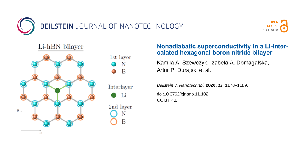
Currently, the most promising research seems to be the properties of the superconducting state in Li-intercalated hexagonal boron nitride bilayer (Li-hBN) compounds. Based on DFT calculations, it has been shown that the critical temperature (TC) of the superconductor–metal phase transition is about 25 K [41] for the Coulomb pseudopotential μ* = 0.14 (identical to the experimental value of μ* obtained for graphene [46]). The expected value of TC is much higher than the maximum temperature that was achieved in graphene intercalated with alkali metals (TC = 8.1 K in Ca-intercalated bilayer graphene) [5]. Also, this value is higher than that of other superconducting low-dimensional structures, e.g., TC ≈ 20 K for a Li- and Na-intercalated blue phosphorene bilayer [47], TC ≈ 16.5 K for a Li-intercalated black phosphorene bilayer [48], and TC≈ 10 K for a Li–MoS2 bilayer [49]. The obtained result for Li-hBN is explained by the relatively high value of the electronic density of states at the Fermi level and the significant contribution to the pairing interaction from the inter-layer electron–phonon coupling [41]. This is due to the formation of characteristic bonds connecting two boron atoms in the upper and lower layers of hBN, which results from the low electronegativity of boron atoms.
From the experimental point of view, it is worth paying attention to the results of research conducted in 2019 by S. Moriyama and co-workers [50]. A superconducting state has been observed in a system consisting of non-twisted bilayer graphene (BLG) and hexagonal boron nitride layers (hBN/BLG/hBN). The following characteristic temperatures were obtained: Tonset ≈ 50 K, T* ≈ 30 K, and TBKT = 14 K, which correspond the onset of superconductivity (90% of the total transition/normal resistance), the crossover to superconductivity (50% of the normal resistance), and the confinement of vortices, respectively.
The important question is whether the Li-hBN bilayer system yield the high critical temperature that was suggested from DFT calculations (TC = 25 K) [41]. We think that this not the case because electron–phonon interaction in Li-hBN needs to be taken into account together with vertex corrections. This is demonstrated by the very high ratio of λωD/εF ≈ 0.46, where λ = 1.17 is the electron–phonon coupling constant, ωD = 165.56 meV is the Debye frequency, and εF = 417.58 meV represents the Fermi energy [41]. Thus, in the presented paper, we characterized the properties of the superconducting state in a Li-hBN bilayer in the framework of the Eliashberg formalism, which includes the vertex corrections of electron–phonon interaction [51]. We compared the results with those obtained using the classical Migdal–Eliashberg theory [52]. Note that the use of the Eliashberg formalism is associated with the high value of the electron–phonon coupling constant λ, which characterizes the superconducting state in Li-hBN [41]. Let us remind that the BCS theory gives the correct results only in the weak-coupling limit, where λ < 0.3 [53,54]. The scope of applicability of the Migdal–Eliashberg theory is carefully discussed in [55].
Theoretical Model
The classical Migdal–Eliashberg (ME) formalism [52,56] represents the natural generalization of the BCS theory (the first microscopic theory of the superconducting state) [53,54]. This generalization takes into account the retardation and strong-coupling effects of the electron–phonon interaction, which are responsible for the condensation of electrons in Cooper pairs [57]. As part of the Eliashberg formalism, the electron–phonon interaction is quantified by the so-called Eliashberg function (α2F(ω)). The form of the Eliashberg function for a specific physical system can be determined theoretically through DFT calculations [58], or experimentally using the data provided by tunnel experiments [59,60]. The electron correlations (the screened Coulomb interaction) are modeled parametrically defining the so-called Coulomb pseudopotential (μ*) [61]. The Eliashberg function and μ* are the only input parameters of the isotropic Eliashberg equations.
The classical Eliashberg equations are thoroughly discussed in the literature [62]. They allow for the self-consistent determination of the superconducting order parameter (Δn = Δ(iωn) and the wave function renormalization factor (Zn = Z(iωn), with an accuracy of the second order relative to the electron–phonon coupling function (g). The symbol ωn = πkBT(2n + 1) defines the fermionic Matsubara frequency. In the case of the phonon-induced superconducting state, the limitation of considerations to the order of g2 is justified by the Migdal theorem [56]. The Migdal theorem applies when the ratio λωD/εF is of the order of 0.01. This means that the energy of the phonons is so small that the vertex corrections for the electron–phonon interaction are irrelevant.
According to DFT calculations, the value of the ratio λωD/εF for Li-hBN is 0.46. This is why the superconducting state in Li-hBN cannot be quantified in the classical Eliashberg theory. The unusually high value of the λωD/εF ratio for Li-hBN is related to the fact that the physical system is quasi-two-dimensional. In the case of the bulk superconductor, the width of the electron band is significantly broadened, which results in the increase of the Fermi energy (εF = 1.63 eV). In addition, the electron–phonon coupling constant decreases (λ = 0.66). As a result, λωD/εF is only 0.07. The calculations carried out by us within the Migdal–Eliashberg formalism prove that the superconducting state has a significantly lower critical temperature value in the bulk than in the quasi-two-dimensional system. In particular, we obtained TC ∈ {14.01, 8.64, 4.6} K, for μ* ∈ {0.1, 0.2, 0.3}, respectively.
To realize how uncommonly high the value of λωD/εF for Li-hBN is, it is enough to note that for the Li–MoS2 bilayer, we obtain λωD/εF = 0.15 [49]. In bilayers of black and blue phosphorus intercalated with lithium, λωD/εF is equal to 0.05 and 0.1, respectively [47,48]. A value of λωD/εF of 0.09 causes a noticeable modification of the properties of the superconducting state, as in the case of LiC6, where TC ≈ 6 K [2,46,63,64].
Therefore, to describe the superconducting state in Li-hBN, we used the Eliashberg equations derived with an accuracy of the fourth order relative to g (lowest-order vertex corrections, LOVC). These equations were derived by Freericks et al. [51] to analyze the properties of the superconducting state in lead. They take the form given in Equation 1 and Equation 2 (A = 1):
(1)(2)
while for A = 0, we get the classic Migdal–Eliashberg equations. The order parameter is given by the formula Δn = φn/Zn. The symbol λn,m represents the pairing kernel for the electron–phonon interactions:
(3)
The Coulomb pseudopotential function is: , where θ(x) is the Heaviside function, and ωc represents the cut-off frequency (ωc = 3ωD = 496.7 meV).
Freericks’ equations allow one to determine the values of the order parameter and the wave function renormalization factor in a self-consistent manner, which is undoubtedly their great advantage. These are isotropic equations, which means that the self-consistent procedure does not apply to the electron momentum (k). From the physical point of view this should not be significant, because the phonon-induced superconducting state is highly isotropic [62]. The situation would of course change radically if, in addition, the strong electron correlations had to be taken into account. Eliashberg equations including vertex corrections and an explicit dependence on k are also given in the literature [65-67]. These equations were derived in the context of research on the superconducting state in fullerene systems [68,69], in high-TC cuprates [70-72], in heavy fermion compounds [73], and in superconductors under high magnetic fields [74]. Unfortunately, due to enormous mathematical difficulties, their full self-consistent solutions are still unknown (Δn,k and Zn,k).
Also, Freericks’ equations have been recently successfully used to analyze the superconducting state with high critical temperature values in compounds such as PH3 (TC ≈ 80 K), H3S (TC ≈ 200 K) [75], and H2S (TC ≈ 35 K) [76].
From the mathematical point of view, the Eliashberg equations are solved in a self-consistent manner taking into account the correspondingly large number of fermionic Matsubara frequencies [77,78]. In our considerations, we assumed that this number (M) is 4000, which ensured the appropriate convergence of solutions of the Eliashberg equations for a temperature higher or equal to T0 = 4 K. Due to the lack of experimental data in the examined physical system we took into account the Coulomb pseudopotential in a range from 0.1 to 0.2, while the value of 0.14 was already considered in [41].
Results
In Figure 1, we plotted the dependence of the order parameter on the temperature. Note that under the imaginary axis formalism, it is assumed that the physical value of the order parameter is Δn=1. In the classic ME model, we obtained the following critical temperature values: ∈ {31.9, 26.9, 21} K, respectively, for μ* ∈ {0.1, 0.14, 0.2}. Comparing the obtained results with the results taking into account the impact of the vertex corrections, ∈ {19.1,15.5,11.8} K), we find that the nonadiabatic superconducting state in Li-hBN has a much lower value of TC than it would follow from the ME model.
Figure 1:
The order parameter as a function of the temperature. ME model - symbols with the dot, LOVC model - empty symbols, μ* ∈ {0.1, 0.14, 0.2}. The solid lines represent the parameterization of numerical results using Equation 6. The dashed lines were obtained as part of the BCS theory (mean-field theory).
Figure 1:
The order parameter as a function of the temperature. ME model - symbols with the dot, LOVC model -...
The observed lowering of the critical temperature value does not only result from the static corrections (Stat.), a good measure of which is the ratio m = ωD/εF = 0.4 (Migdal parameter). It is also associated with dynamic corrections modeled by the explicit dependence of the order parameter and the wave function renormalization factor on the Matsubara frequency. Based on the results of [67,79], the impact of static vertex corrections on the critical temperature can be estimated using the formula
(4)
where is the critical temperature value calculated on the basis of the Allen–Dynes formula [80]. The input from the static part of the vertex corrections has the form
(5)
A good measure of the dynamic vertex corrections is
The results are summarized in Table 1. As one can see, the static part of the vertex corrections is responsible for 80–90% of the difference in TC.
Table 1:
Critical temperature estimated from the LOVC model, from the ME model, using the Allen–Dynes formula [80], and from the analytical model including static corrections (). Additionally, the values of the D parameter were given.
μ*
(K)
(K)
(K)
(K)
D%
0.1
19.1
31.9
32.2
21.4
18
0.14
15.5
26.9
26.7
17.8
20.2
0.2
11.8
21
19.4
12.9
12
The numerical results obtained from the Eliashberg equations can be parameterized using the formula [81]
(6)
where Δ(0) = Δ(T0). Using the LOVC model, we obtained Γ ∈ {2.17, 2.2, 2.8}, respectively, for μ* ∈ {0.1, 0.14, 0.2}. The exponent Γ for the classic ME approach differs significantly in values, i.e., Γ∈ {3.45, 3.4, 3.45}, respectively. The accuracy of analytical parameterization of the numerical results is presented in Figure 1 (solid lines). In addition, the results obtained under the mean-field BCS model are given by the dashed lines. In this case, Δ(0) = 1.76·kBTC was adopted [53,54]. The value of the exponent Γ for the BCS model is 3 [81].
Note the differences in the shape of the curves corresponding to the parameterization of the Eliashberg results and the BCS theory. In the case of the ME model, the differences result only from retardation and strong-coupling effects correctly taken into account in the ME formalism. These effects can be characterized by calculating the value of the ratio r = kBTC/ωln, where
is the logarithmic phonon frequency [80]. The r parameter for Li-hBN is rME∈ {0.095, 0.08, 0.062 } or rLOVC∈ {0.057, 0.046, 0.035}, respectively, for μ* ∈ {0.1, 0.14, 0.2}. This means that the effects considered are significant even when we consider the vertex corrections for the electron–phonon interaction. Also note that retardation and strong-coupling effects for Li-hBN are of the same order as in Li-MoS2 bilayer compounds [49], Li-black phosphorene bilayers [48], and Li-blue phosphorene bilayers [47], i.e., 0.068, 0.094, and 0.099, respectively. These results were obtained for TC determined from the Allen–Dynes formula [80] assuming μ* = 0.1. In the BCS limit, the Eliashberg equations predict r→0.
In the LOVC theory, we take into account the vertex corrections as well as the retardation and strong-coupling effects. As a result, the differences between the Eliashberg parameterization curves and the BCS curves noticeably increase. A good measure of this effect is the value of the ratio RΔ = 2Δ(0)/kBTC. For the Li-hBN system, we obtained ∈ {4.6, 4.29, 3.99} and ∈ {4.12, 4.04, 3.9}. It should be emphasized that using BCS theory, a value of RΔ = 3.53 is obtained. It is the universal constant of the model [53,54]. The results obtained for μ* ∈ ⟨0.1, 0.2⟩ are presented in Figure 2. One can notice an interesting effect, namely, that with the increase of depairing electron correlations, the impact of vertex corrections on the ratio RΔ decreases, i.e., for μ* ≈ 0.2 the parameter differs only slightly from .
Figure 2:
The values of the ratio RΔ as a function of the Coulomb pseudopotential. The results obtained under the model: LOVC, ME, and BCS.
Figure 2:
The values of the ratio RΔ as a function of the Coulomb pseudopotential. The results obtained under...
Knowing the full dependence of the order parameter on the Matsubara frequency, we determined the normalized density of states:
(7)
where the pair breaking parameter δ equals 0.15 meV. We calculated the value of Δ(ω) by continuing the function Δn on the real axis [82]. The results obtained by using the LOVC approach for NS(ω)/NN(ω) are given in Figure 3a–c. The presented curves can also be determined on the basis of the data obtained using the tunneling junction. Hence, any experimental results directly relate to the predictions of the Eliashberg formalism taking into account the effect of vertex corrections. Additionally, in Figure 3d–f we plotted the form of the order parameter on the real axis (T = 4 K). The real part of the function Δ(ω) specifies the physical value of the order parameter, which can be calculated using the equation Δ(T) = Re[Δ(ω = Δ(T))] [62]. In the present case, we obtained values that differ from Δn=1 by no more than 10−2%. This result proves that the analytical continuation was correct. The imaginary part of Δ(ω) determines the damping effects. One can see that at low frequencies, where Im[Δ(ω)] = 0, these effects do not occur. From the physical point of view, this means the infinite lifetime of the Cooper pairs. Above the frequency ω ≈ 15 meV, both the real and imaginary part of the order parameter function have a complicated course. This fact results directly from the complicated shape of the Eliashberg function, which models the electron–phonon interaction in the Li-hBN system.
Figure 3:
(a–c) Normalized density of states for the given temperatures. (d–f) The form of the order parameter on the real axis calculated for T = 4 K. The results were obtained in the framework of the LOVC model.
Figure 3:
(a–c) Normalized density of states for the given temperatures. (d–f) The form of the order paramete...
Let us now discuss the effect of vertex corrections on the electron band mass (me). To do this, it is necessary to use the formula , where is the effective electron mass.
The results obtained on the basis of the Eliashberg equations are presented in Figure 4. It is easy to see that the effective mass of the electron is almost twice as high as the electron band mass, with depending very slightly on the temperature. The vertex corrections lower the value of compared to the value predicted under ME formalism. If the temperature equals the critical temperature, this effect can be characterized analytically. Based on Equation 2, we obtained
(8)
Hence,
(9)
where . We see that the lowest-order vertex corrections lower the effective mass the a greater extent when λ and ωD are higher. It should be noted that in this case the critical temperature also increases. The values of and , calculated on the basis of Equation 9, have been marked on Figure 4 using black spheres. We obtained a good agreement between numerical and analytical results.
Figure 4:
The ratio of the electron effective mass to the electron band mass as a function of temperature. The results were obtained in the framework of LOVC model, ME model, and Equation 9. The lines for ME results can be reproduced using the formula: = [Zn=1(TC) − Zn=1(0)](T/TC)Γ + Zn=1(0), where Zn=1(0) = Zn=1(T0).
Figure 4:
The ratio of the electron effective mass to the electron band mass as a function of temperature. Th...
A characterization of the superconducting state in Li-hBN was carried out with the help of the Eliashberg formalism taking into account the lowest-order vertex corrections. Due to the very high value of the ratio λωD/εF, the question regarding the significance of higher-order vertex corrections arises. It turns out that no general answer can be given, as this would require the self-consistent solution of the Eliashberg equations taking into account the vertex corrections of all orders. However, one can give arguments that support the results presented in this paper:
(1) First of all, it should be noted that the very high value of the ratio λωD/εF does not mean that higher-order vertex corrections are equally or even more important than the lowest-order corrections. This is because the renormalization of the bare vertex amplitude g has the form [66]:
(10)
where the functions pj(q,ω) characterize the dependence of the vertex corrections on the momentum (q) and the frequency (ω) of the outgoing phonon. This means that not only the value of the ratio λωD/εF is important, but also the values of all functions pj(q,ω).
(2) The significance of the presented results can be thoroughly understood by analyzing the normal state within the LOVC model. In this case, the self-energy Σ(iωn) depends only on the wave function renormalization factor, because for a temperature equal to or higher than the critical temperature, the order parameter disappears. The values of the wave function renormalization factor obtained by us are easiest to analyze taking into account Equation 9, which should be written as
(11)
where
For the assumed values of the Coulomb pseudopotential, the parameter γ is in the range from 0.323 to 0.331. Therefore, for Li-hBN it is not high enough to lower below 1, which would indicate the loss of stability of the examined compound [83].
Regarding literature results based on models that include the lowest-order vertex corrections [67,84-86], the sign of determined parameter γ is correct. This means that the static contribution of the vertex corrections to the normal self-energy has been qualitatively calculated in an appropriate manner. Due to the fact that Equation 9 reproduces well the numerical results (see Figure 4), the same can also be said about the self-consistent results. However, the values of the parameter γ for the models analyzed in [85] may differ significantly, which is associated with the assumed approximations. Our result is comparable with the estimates based on [67,85], where the γ parameter is equal to 0.317. However, it is lower than the values of 0.547, 0.685 and 1.07 that are obtained on the basis of [84-86]. On the other hand, the parameter γ determined by us exceeds the value of γW = 0.034 [87], which was obtained based on the Ward identity [85,88,89]. Note that Ward-type identities result from the conservation of the total charge and the total spin of fermions, as a result of which one can obtain the exact relationships between the self-energy and the vertex corrections. Nevertheless, the Ward identity considered in the context of superconducting states is an equation for two functions (scalar and vector) and, thus, allows for multiple solutions. Therefore, based on the results presented in [85,90-92] one can obtain the opposite value γ = −0.9.
To sum up, the presented LOVC model predicts a small decrease in the value of the wave function renormalization factor relative to other approaches based on the lowest-order vertex corrections. This result reduces the risk of stability loss of the examined system as a result of taking into account higher-order corrections. The estimated values of the parameter γ are very close to the value based on [67,85], and are higher than γW, with the reservations made regarding the method based on the Ward identity.
(3) It is very difficult to justify our results for the values of temperatures lower than TC, where self-consistent calculations are required for φn and Zn. Hence, we discuss the impact on our predictions of vertex corrections of the order of g6 (which corresponds to λ3). Due to the very complicated form of the considered contributions, we take into account the case |TC − T| ≪ TC. This approach allows us to linearize the Eliashberg equations [62], which greatly simplifies the numerical analysis [77]. The contributions of the order of g6 to the Eliashberg equations were determined by using the Green thermodynamic formalism [93]. Note that the Migdal–Eliashberg approximation is based on the replacement of the mixed Green’s function
by the product of the full electron Green’s function Gk(iωn)(iωn) and the phonon propagator for the non-interacting phonons:
We have extended this step. In particular, we have strictly determined the equation of motion for Fk,q,q'(iωn)(iωn), and then repeated the procedure for all new unknown functions. Finally, based on the Wick theorem [94], we closed the obtained system of equations. The contribution of the order of g6 to the first Eliashberg equation can be written as presented in Equation 12. In the case of the equation for the wave function renormalization factor we obtained the expression in Equation 13.
(12)(13)
The explicit expressions for the kernels are given below:
(14)(15)(16)(17)(18)(19)(20)
In Equation 14–Equation 20, gq means the electron–phonon matrix element, ωq represents the phonon energy, and εk is the electron band energy. In addition, means the Fermi–Dirac function and is the Bose–Einstein function. The symbol
represents the higher-order phonon Green’s function. It was designated by us assuming no interaction between phonons. The function Dk(ωm) is given by the formula
The isotropic form of contributions of the order λ3 (Equation 12 and Equation 13) was obtained by exchanging the wave vector summation by the energy integration with constant density of states, wherein some integrals can be calculated numerically. We do not give the explicit isotropic expressions, because they are very extensive. We performed numerical calculations for all considered values of the Coulomb pseudopotential. For μ* ∈ {0.1, 0.14, 0.2}, we obtained a reduction of the critical temperature , respectively, by 6.2%, 5.4% and 4.7%. This means that the vertex corrections of the order of λ3 do not significantly change the critical temperature values determined with the lowest-order vertex corrections. In our opinion, the analysis presented above clearly suggests that the critical temperature in Li-hBN is lower than .
In the last paragraph of this section, we discuss a possible way to increase the value of the critical temperature in Li-hBN. We believe that this is possible. To do this, consider the form of the Eliashberg function of Li-hBN (Figure 5). It can easily be seen that the Eliashberg function consists of two clearly separated parts (similar to the functions of hydrogen compounds [95,96]). In the low-frequency range (ω ∈ {4.59, 93.29} meV) nitrogen and boron contributions are important. In the frequency range from 145.16 to 176.13 meV, the electron–phonon interaction associated with lithium atoms dominates. These frequency ranges are separable, with the Eliashberg function taking very small values in the range from 93.29 to 145.16 meV. The above facts suggest that the composition of Li-hBN could be changed to significantly increase the values of the Eliashberg function in the range from 93.29 to 145.16 meV. Most likely by appropriate doping of the starting compound. However, this is not a simple task and requires DFT calculations.
Figure 5:
Eliashberg function α2F(ω) and electron–phonon coupling function for Li-hBN. The results were obtained in [41]. The figure also indicates the contributions from nitrogen, boron and lithium, λN = 0.82, λB = 0.25, and λLi = 0.1, where λN + λB + λLi = 1.17.
Figure 5:
Eliashberg function α2F(ω) and electron–phonon coupling function for Li-hBN. The results were obta...
Also striking is the possibility of substitution (at least partially) of lithium by hydrogen or of boron and nitrogen by heavier elements. In the first case, the increase in critical temperature could be associated with an increase of the Debye frequency (TC ∼ ωD and , while the hydrogen nucleus has a lower mass than the lithium nucleus). In the second case, the increase in TC could result from the increase in the electron–phonon coupling constant (TC ∼ exp(−1/λ). Contributions from heavier elements in the Eliashberg function are in the low-frequency range and are potentially more significant for λ. To find out, note that the electron–phonon coupling constant is defined by .
Conclusion
The superconducting state in Li-hBN is induced by electron–phonon interaction, which is characterized by the uncommonly high value of the ratio λωD/εF = 0.46. This means that the thermodynamic properties of the superconducting phase should be determined using a formalism explicitly including vertex corrections. Note that the very high value of the ratio λωD/εF is related to the quasi-two-dimensionality of considered system [41].
We showed that nonadiabatic effects significantly lower the critical temperature ( ∈ {19.1, 15.5, 11.8} K), compared to the results obtained in the framework of the Migdal–Eliashberg theory, ∈ {31.9, 26.9, 21} K, for μ* ∈ {0.1, 0.14, 0.2}, respectively. In our opinion, there is no reason to believe that the critical temperature in Li-hBN exceeds 20 K, which certainly limits its applications. The vertex corrections of the order of λ3 slightly decrease .
Note that the low values of TC occur in principle in the whole family of systems in which a honeycomb crystal structure plays an important role [5,47-49]. This structure, although fundamental for the properties of graphene, is unfavorable regarding superconducting states. The reason for this is that the van Hove singularity in the electronic density of states is considerably distant form the Fermi level [97]. This is not the case for a square lattice, where the van Hove singularity is very close or even at the Fermi level, which means that the value of TC can increase by one order of magnitude [98].
Finally, let us note that from the point of view of fundamental research on phonon-induced superconducting states, the Li-hBN system seems to be very interesting because of the unusually high value of the ratio λωD/εF, which is comparable to the value obtained for fullerene compounds [66,68]. Therefore, Li-hBN can be used to test the predictions of future theories that include vertex corrections in a fully self-consistent manner (both Matsubara frequencies and the electron wave vector k). We are currently investigating this issue extensively. Preliminary results for the ME formalism can be found in [99,100].
Acknowledgements
The authors would like to thank Nao H. Shimada, Emi Minamitani, and Satoshi Watanabe (University of Tokyo) for providing data on the Eliashberg function for Li-hBN bilayer, presented in [41], and for providing information on the electronic structure of bulk Li-hBN.
References
Ohta, T.; Bostwick, A.; Seyller, T.; Horn, K.; Rotenberg, E. Science2006,313, 951–954. doi:10.1126/science.1130681
Return to citation in text:
[1]
Profeta, G.; Calandra, M.; Mauri, F. Nat. Phys.2012,8, 131–134. doi:10.1038/nphys2181
Return to citation in text:
[1]
[2]
Pešić, J.; Gajić, R.; Hingerl, K.; Belić, M. EPL2014,108, 67005. doi:10.1209/0295-5075/108/67005
Return to citation in text:
[1]
Guzman, D. M.; Alyahyaei, H. M.; Jishi, R. A. 2D Mater.2014,1, 021005. doi:10.1088/2053-1583/1/2/021005
Return to citation in text:
[1]
Margine, E. R.; Lambert, H.; Giustino, F. Sci. Rep.2016,6, 21414. doi:10.1038/srep21414
Return to citation in text:
[1]
[2]
[3]
Liu, H.; Neal, A. T.; Zhu, Z.; Luo, Z.; Xu, X.; Tománek, D.; Ye, P. D. ACS Nano2014,8, 4033–4041. doi:10.1021/nn501226z
Return to citation in text:
[1]
Shikin, A. M.; Prudnikova, G. V.; Adamchuk, V. K.; Moresco, F.; Rieder, K.-H. Phys. Rev. B2000,62, 13202–13208. doi:10.1103/physrevb.62.13202
Return to citation in text:
[1]
Rosei, R.; De Crescenzi, M.; Sette, F.; Quaresima, C.; Savoia, A.; Perfetti, P. Phys. Rev. B1983,28, 1161–1164. doi:10.1103/physrevb.28.1161
Return to citation in text:
[1]
Shikin, A. M.; Farías, D.; Rieder, K. H. Europhys. Lett.1998,44, 44–49. doi:10.1209/epl/i1998-00432-x
Return to citation in text:
[1]
Dedkov, Y. S.; Shikin, A. M.; Adamchuk, V. K.; Molodtsov, S. L.; Laubschat, C.; Bauer, A.; Kaindl, G. Phys. Rev. B2001,64, 035405. doi:10.1103/physrevb.64.035405
Return to citation in text:
[1]
Brugger, T.; Günther, S.; Wang, B.; Dil, J. H.; Bocquet, M.-L.; Osterwalder, J.; Wintterlin, J.; Greber, T. Phys. Rev. B2009,79, 045407. doi:10.1103/physrevb.79.045407
Return to citation in text:
[1]
Moritz, W.; Wang, B.; Bocquet, M.-L.; Brugger, T.; Greber, T.; Wintterlin, J.; Günther, S. Phys. Rev. Lett.2010,104, 136102. doi:10.1103/physrevlett.104.136102
Return to citation in text:
[1]
Land, T. A.; Michely, T.; Behm, R. J.; Hemminger, J. C.; Comsa, G. Surf. Sci.1992,264, 261–270. doi:10.1016/0039-6028(92)90183-7
Return to citation in text:
[1]
Starr, D. E.; Pazhetnov, E. M.; Stadnichenko, A. I.; Boronin, A. I.; Shaikhutdinov, S. K. Surf. Sci.2006,600, 2688–2695. doi:10.1016/j.susc.2006.04.035
Return to citation in text:
[1]
[2]
Forbeaux, I.; Themlin, J.-M.; Debever, J.-M. Phys. Rev. B1998,58, 16396–16406. doi:10.1103/physrevb.58.16396
Return to citation in text:
[1]
Mendes-de-Sa, T. G.; Goncalves, A. M. B.; Matos, M. J. S.; Coelho, P. M.; Magalhaes-Paniago, R.; Lacerda, R. G. Nanotechnology2012,23, 475602. doi:10.1088/0957-4484/23/47/475602
Return to citation in text:
[1]
Hass, J.; Varchon, F.; Millán-Otoya, J. E.; Sprinkle, M.; Sharma, N.; de Heer, W. A.; Berger, C.; First, P. N.; Magaud, L.; Conrad, E. H. Phys. Rev. Lett.2008,100, 125504. doi:10.1103/physrevlett.100.125504
Return to citation in text:
[1]
Chen, J.-H.; Jang, C.; Xiao, S.; Ishigami, M.; Fuhrer, M. S. Nat. Nanotechnol.2008,3, 206–209. doi:10.1038/nnano.2008.58
Return to citation in text:
[1]
Lee, D. S.; Riedl, C.; Krauss, B.; von Klitzing, K.; Starke, U.; Smet, J. H. Nano Lett.2008,8, 4320–4325. doi:10.1021/nl802156w
Return to citation in text:
[1]
Geringer, V.; Liebmann, M.; Echtermeyer, T.; Runte, S.; Schmidt, M.; Rückamp, R.; Lemme, M. C.; Morgenstern, M. Phys. Rev. Lett.2009,102, 076102. doi:10.1103/physrevlett.102.076102
Return to citation in text:
[1]
Ponomarenko, L. A.; Geim, A. K.; Zhukov, A. A.; Jalil, R.; Morozov, S. V.; Novoselov, K. S.; Grigorieva, I. V.; Hill, E. H.; Cheianov, V. V.; Fal’ko, V. I.; Watanabe, K.; Taniguchi, T.; Gorbachev, R. V. Nat. Phys.2011,7, 958–961. doi:10.1038/nphys2114
Return to citation in text:
[1]
[2]
Nagashima, A.; Tejima, N.; Gamou, Y.; Kawai, T.; Oshima, C. Phys. Rev. Lett.1995,75, 3918–3921. doi:10.1103/physrevlett.75.3918
Return to citation in text:
[1]
Novoselov, K. S.; Jiang, D.; Schedin, F.; Booth, T. J.; Khotkevich, V. V.; Morozov, S. V.; Geim, A. K. Proc. Natl. Acad. Sci. U. S. A.2005,102, 10451–10453. doi:10.1073/pnas.0502848102
Return to citation in text:
[1]
Decker, R.; Wang, Y.; Brar, V. W.; Regan, W.; Tsai, H.-Z.; Wu, Q.; Gannett, W.; Zettl, A.; Crommie, M. F. Nano Lett.2011,11, 2291–2295. doi:10.1021/nl2005115
Return to citation in text:
[1]
Giovannetti, G.; Khomyakov, P. A.; Brocks, G.; Kelly, P. J.; van den Brink, J. Phys. Rev. B2007,76, 073103. doi:10.1103/physrevb.76.073103
Return to citation in text:
[1]
Dean, C. R.; Young, A. F.; Meric, I.; Lee, C.; Wang, L.; Sorgenfrei, S.; Watanabe, K.; Taniguchi, T.; Kim, P.; Shepard, K. L.; Hone, J. Nat. Nanotechnol.2010,5, 722–726. doi:10.1038/nnano.2010.172
Return to citation in text:
[1]
[2]
Britnell, L.; Gorbachev, R. V.; Jalil, R.; Belle, B. D.; Schedin, F.; Mishchenko, A.; Georgiou, T.; Katsnelson, M. I.; Eaves, L.; Morozov, S. V.; Peres, N. M. R.; Leist, J.; Geim, A. K.; Novoselov, K. S.; Ponomarenko, L. A. Science2012,335, 947–950. doi:10.1126/science.1218461
Return to citation in text:
[1]
Haigh, S. J.; Gholinia, A.; Jalil, R.; Romani, S.; Britnell, L.; Elias, D. C.; Novoselov, K. S.; Ponomarenko, L. A.; Geim, A. K.; Gorbachev, R. Nat. Mater.2012,11, 764–767. doi:10.1038/nmat3386
Return to citation in text:
[1]
Dean, C.; Young, A. F.; Wang, L.; Meric, I.; Lee, G.-H.; Watanabe, K.; Taniguchi, T.; Shepard, K.; Kim, P.; Hone, J. Solid State Commun.2012,152, 1275–1282. doi:10.1016/j.ssc.2012.04.021
Return to citation in text:
[1]
Ponomarenko, L. A.; Gorbachev, R. V.; Yu, G. L.; Elias, D. C.; Jalil, R.; Patel, A. A.; Mishchenko, A.; Mayorov, A. S.; Woods, C. R.; Wallbank, J. R.; Mucha-Kruczynski, M.; Piot, B. A.; Potemski, M.; Grigorieva, I. V.; Novoselov, K. S.; Guinea, F.; Fal’ko, V. I.; Geim, A. K. Nature2013,497, 594–597. doi:10.1038/nature12187
Return to citation in text:
[1]
Dean, C. R.; Wang, L.; Maher, P.; Forsythe, C.; Ghahari, F.; Gao, Y.; Katoch, J.; Ishigami, M.; Moon, P.; Koshino, M.; Taniguchi, T.; Watanabe, K.; Shepard, K. L.; Hone, J.; Kim, P. Nature2013,497, 598–602. doi:10.1038/nature12186
Return to citation in text:
[1]
Shimada, N. H.; Minamitani, E.; Watanabe, S. Appl. Phys. Express2017,10, 093101. doi:10.7567/apex.10.093101
Return to citation in text:
[1]
[2]
[3]
[4]
[5]
[6]
[7]
[8]
[9]
[10]
Altintas, B.; Parlak, C.; Bozkurt, C.; Eryiğit, R. Eur. Phys. J. B2011,79, 301–312. doi:10.1140/epjb/e2010-10660-4
Return to citation in text:
[1]
Fatemi, V.; Wu, S.; Cao, Y.; Bretheau, L.; Gibson, Q. D.; Watanabe, K.; Taniguchi, T.; Cava, R. J.; Jarillo-Herrero, P. Science2018,362, 926–929. doi:10.1126/science.aar4642
Return to citation in text:
[1]
Fagaly, R. L. Rev. Sci. Instrum.2006,77, 101101. doi:10.1063/1.2354545
Return to citation in text:
[1]
Komatsu, K.; Morita, Y.; Watanabe, E.; Tsuya, D.; Watanabe, K.; Taniguchi, T.; Moriyama, S. Sci. Adv.2018,4, eaaq0194. doi:10.1126/sciadv.aaq0194
Return to citation in text:
[1]
Ludbrook, B. M.; Levy, G.; Nigge, P.; Zonno, M.; Schneider, M.; Dvorak, D. J.; Veenstra, C. N.; Zhdanovich, S.; Wong, D.; Dosanjh, P.; Straßer, C.; Stöhr, A.; Forti, S.; Ast, C. R.; Starke, U.; Damascelli, A. Proc. Natl. Acad. Sci. U. S. A.2015,112, 11795–11799. doi:10.1073/pnas.1510435112
Return to citation in text:
[1]
[2]
Freericks, J. K.; Nicol, E. J.; Liu, A. Y.; Quong, A. A. Phys. Rev. B1997,55, 11651–11658. doi:10.1103/physrevb.55.11651
Return to citation in text:
[1]
[2]
Eliashberg, G. M. Sov. Phys. - JETP1960,11, 696.
Return to citation in text:
[1]
[2]
Bardeen, J.; Cooper, L. N.; Schrieffer, J. R. Phys. Rev.1957,106, 162–164. doi:10.1103/physrev.106.162
Return to citation in text:
[1]
[2]
[3]
[4]
Bardeen, J.; Cooper, L. N.; Schrieffer, J. R. Phys. Rev.1957,108, 1175–1204. doi:10.1103/physrev.108.1175
Return to citation in text:
[1]
[2]
[3]
[4]
Chubukov, A. V.; Abanov, A.; Esterlis, I.; Kivelson, S. A. Ann. Phys. (Amsterdam, Neth.)2020,417, 168190. doi:10.1016/j.aop.2020.168190
Return to citation in text:
[1]
Migdal, A. B. Sov. Phys. - JETP1958,34, 996.
Return to citation in text:
[1]
[2]
Uemura, Y. J.; Le, L. P.; Luke, G. M.; Sternlieb, B. J.; Wu, W. D.; Brewer, J. H.; Riseman, T. M.; Seaman, C. L.; Maple, M. B.; Ishikawa, M.; Hinks, D. G.; Jorgensen, J. D.; Saito, G.; Yamochi, H. Phys. Rev. Lett.1991,66, 2665–2668. doi:10.1103/physrevlett.66.2665
Return to citation in text:
[1]
Uemura, Y. J.; Le, L. P.; Luke, G. M.; Sternlieb, B. J.; Wu, W. D.; Brewer, J. H.; Riseman, T. M.; Seaman, C. L.; Maple, M. B.; Ishikawa, M.; Hinks, D. G.; Jorgensen, J. D.; Saito, G.; Yamochi, H. Phys. Rev. Lett.1992,68, 2712. doi:10.1103/physrevlett.68.2712
Return to citation in text:
[1]
d'Ambrumenil, N. Nature1991,352, 472–473. doi:10.1038/352472a0
Return to citation in text:
[1]
Wojciechowski, R. J. On the validity of the Migdal’s theorem in the heavy fermion systems. International Centre For Theoretical Physics, Trieste; International Atomic Energy Agency, 1996; Vol. 28.
Return to citation in text:
[1]
Profeta, G.; Calandra, M.; Mauri, F. Nat. Phys.2012,8, 131–134. doi:10.1038/nphys2181
46.
Ludbrook, B. M.; Levy, G.; Nigge, P.; Zonno, M.; Schneider, M.; Dvorak, D. J.; Veenstra, C. N.; Zhdanovich, S.; Wong, D.; Dosanjh, P.; Straßer, C.; Stöhr, A.; Forti, S.; Ast, C. R.; Starke, U.; Damascelli, A. Proc. Natl. Acad. Sci. U. S. A.2015,112, 11795–11799. doi:10.1073/pnas.1510435112
Uemura, Y. J.; Le, L. P.; Luke, G. M.; Sternlieb, B. J.; Wu, W. D.; Brewer, J. H.; Riseman, T. M.; Seaman, C. L.; Maple, M. B.; Ishikawa, M.; Hinks, D. G.; Jorgensen, J. D.; Saito, G.; Yamochi, H. Phys. Rev. Lett.1991,66, 2665–2668. doi:10.1103/physrevlett.66.2665
71.
Uemura, Y. J.; Le, L. P.; Luke, G. M.; Sternlieb, B. J.; Wu, W. D.; Brewer, J. H.; Riseman, T. M.; Seaman, C. L.; Maple, M. B.; Ishikawa, M.; Hinks, D. G.; Jorgensen, J. D.; Saito, G.; Yamochi, H. Phys. Rev. Lett.1992,68, 2712. doi:10.1103/physrevlett.68.2712
Wojciechowski, R. J. On the validity of the Migdal’s theorem in the heavy fermion systems. International Centre For Theoretical Physics, Trieste; International Atomic Energy Agency, 1996; Vol. 28.
Land, T. A.; Michely, T.; Behm, R. J.; Hemminger, J. C.; Comsa, G. Surf. Sci.1992,264, 261–270. doi:10.1016/0039-6028(92)90183-7
23.
Starr, D. E.; Pazhetnov, E. M.; Stadnichenko, A. I.; Boronin, A. I.; Shaikhutdinov, S. K. Surf. Sci.2006,600, 2688–2695. doi:10.1016/j.susc.2006.04.035
Dedkov, Y. S.; Shikin, A. M.; Adamchuk, V. K.; Molodtsov, S. L.; Laubschat, C.; Bauer, A.; Kaindl, G. Phys. Rev. B2001,64, 035405. doi:10.1103/physrevb.64.035405
Ludbrook, B. M.; Levy, G.; Nigge, P.; Zonno, M.; Schneider, M.; Dvorak, D. J.; Veenstra, C. N.; Zhdanovich, S.; Wong, D.; Dosanjh, P.; Straßer, C.; Stöhr, A.; Forti, S.; Ast, C. R.; Starke, U.; Damascelli, A. Proc. Natl. Acad. Sci. U. S. A.2015,112, 11795–11799. doi:10.1073/pnas.1510435112
Starr, D. E.; Pazhetnov, E. M.; Stadnichenko, A. I.; Boronin, A. I.; Shaikhutdinov, S. K. Surf. Sci.2006,600, 2688–2695. doi:10.1016/j.susc.2006.04.035
Novoselov, K. S.; Jiang, D.; Schedin, F.; Booth, T. J.; Khotkevich, V. V.; Morozov, S. V.; Geim, A. K. Proc. Natl. Acad. Sci. U. S. A.2005,102, 10451–10453. doi:10.1073/pnas.0502848102
Ponomarenko, L. A.; Geim, A. K.; Zhukov, A. A.; Jalil, R.; Morozov, S. V.; Novoselov, K. S.; Grigorieva, I. V.; Hill, E. H.; Cheianov, V. V.; Fal’ko, V. I.; Watanabe, K.; Taniguchi, T.; Gorbachev, R. V. Nat. Phys.2011,7, 958–961. doi:10.1038/nphys2114
Mendes-de-Sa, T. G.; Goncalves, A. M. B.; Matos, M. J. S.; Coelho, P. M.; Magalhaes-Paniago, R.; Lacerda, R. G. Nanotechnology2012,23, 475602. doi:10.1088/0957-4484/23/47/475602
26.
Hass, J.; Varchon, F.; Millán-Otoya, J. E.; Sprinkle, M.; Sharma, N.; de Heer, W. A.; Berger, C.; First, P. N.; Magaud, L.; Conrad, E. H. Phys. Rev. Lett.2008,100, 125504. doi:10.1103/physrevlett.100.125504
Ponomarenko, L. A.; Gorbachev, R. V.; Yu, G. L.; Elias, D. C.; Jalil, R.; Patel, A. A.; Mishchenko, A.; Mayorov, A. S.; Woods, C. R.; Wallbank, J. R.; Mucha-Kruczynski, M.; Piot, B. A.; Potemski, M.; Grigorieva, I. V.; Novoselov, K. S.; Guinea, F.; Fal’ko, V. I.; Geim, A. K. Nature2013,497, 594–597. doi:10.1038/nature12187
40.
Dean, C. R.; Wang, L.; Maher, P.; Forsythe, C.; Ghahari, F.; Gao, Y.; Katoch, J.; Ishigami, M.; Moon, P.; Koshino, M.; Taniguchi, T.; Watanabe, K.; Shepard, K. L.; Hone, J.; Kim, P. Nature2013,497, 598–602. doi:10.1038/nature12186
Ponomarenko, L. A.; Geim, A. K.; Zhukov, A. A.; Jalil, R.; Morozov, S. V.; Novoselov, K. S.; Grigorieva, I. V.; Hill, E. H.; Cheianov, V. V.; Fal’ko, V. I.; Watanabe, K.; Taniguchi, T.; Gorbachev, R. V. Nat. Phys.2011,7, 958–961. doi:10.1038/nphys2114
Britnell, L.; Gorbachev, R. V.; Jalil, R.; Belle, B. D.; Schedin, F.; Mishchenko, A.; Georgiou, T.; Katsnelson, M. I.; Eaves, L.; Morozov, S. V.; Peres, N. M. R.; Leist, J.; Geim, A. K.; Novoselov, K. S.; Ponomarenko, L. A. Science2012,335, 947–950. doi:10.1126/science.1218461
37.
Haigh, S. J.; Gholinia, A.; Jalil, R.; Romani, S.; Britnell, L.; Elias, D. C.; Novoselov, K. S.; Ponomarenko, L. A.; Geim, A. K.; Gorbachev, R. Nat. Mater.2012,11, 764–767. doi:10.1038/nmat3386
38.
Dean, C.; Young, A. F.; Wang, L.; Meric, I.; Lee, G.-H.; Watanabe, K.; Taniguchi, T.; Shepard, K.; Kim, P.; Hone, J. Solid State Commun.2012,152, 1275–1282. doi:10.1016/j.ssc.2012.04.021


![[2190-4286-11-102-i1]](/bjnano/content/inline/2190-4286-11-102-i1.svg?max-width=590&scale=1.18182)
![[2190-4286-11-102-i2]](/bjnano/content/inline/2190-4286-11-102-i2.svg?max-width=590&scale=1.18182)
![[2190-4286-11-102-i3]](/bjnano/content/inline/2190-4286-11-102-i3.svg?max-width=590&scale=1.18182)
![[Graphic 1]](/bjnano/content/inline/2190-4286-11-102-i21.svg?max-width=637&scale=1.18182) , where θ(x) is the Heaviside function, and ωc represents the cut-off frequency (ωc = 3ωD = 496.7 meV).
, where θ(x) is the Heaviside function, and ωc represents the cut-off frequency (ωc = 3ωD = 496.7 meV).![[Graphic 2]](/bjnano/content/inline/2190-4286-11-102-i22.svg?max-width=637&scale=1.18182) ∈ {31.9, 26.9, 21} K, respectively, for μ* ∈ {0.1, 0.14, 0.2}. Comparing the obtained results with the results taking into account the impact of the vertex corrections,
∈ {31.9, 26.9, 21} K, respectively, for μ* ∈ {0.1, 0.14, 0.2}. Comparing the obtained results with the results taking into account the impact of the vertex corrections, ![[Graphic 3]](/bjnano/content/inline/2190-4286-11-102-i23.svg?max-width=637&scale=1.18182) ∈ {19.1,15.5,11.8} K), we find that the nonadiabatic superconducting state in Li-hBN has a much lower value of TC than it would follow from the ME model.
∈ {19.1,15.5,11.8} K), we find that the nonadiabatic superconducting state in Li-hBN has a much lower value of TC than it would follow from the ME model.![[2190-4286-11-102-1]](/bjnano/content/figures/2190-4286-11-102-1.png?scale=2.0&max-width=1024&background=FFFFFF)
![[2190-4286-11-102-i4]](/bjnano/content/inline/2190-4286-11-102-i4.svg?max-width=590&scale=1.18182)
![[Graphic 4]](/bjnano/content/inline/2190-4286-11-102-i24.svg?max-width=637&scale=1.18182) is the critical temperature value calculated on the basis of the Allen–Dynes formula [80]. The input from the static part of the vertex corrections has the form
is the critical temperature value calculated on the basis of the Allen–Dynes formula [80]. The input from the static part of the vertex corrections has the form![[2190-4286-11-102-i5]](/bjnano/content/inline/2190-4286-11-102-i5.svg?max-width=590&scale=1.18182)
![[Graphic 5]](/bjnano/content/inline/2190-4286-11-102-i25.svg?max-width=637&scale=1.18182)
![[Graphic 6]](/bjnano/content/inline/2190-4286-11-102-i26.svg?max-width=637&scale=1.18182) ). Additionally, the values of the D parameter were given.
). Additionally, the values of the D parameter were given.
![[Graphic 7]](/bjnano/content/inline/2190-4286-11-102-i27.svg?max-width=637&scale=1.0) (K)
(K)
![[Graphic 8]](/bjnano/content/inline/2190-4286-11-102-i28.svg?max-width=637&scale=1.0) (K)
(K)
![[Graphic 9]](/bjnano/content/inline/2190-4286-11-102-i29.svg?max-width=637&scale=1.0) (K)
(K)
![[Graphic 10]](/bjnano/content/inline/2190-4286-11-102-i30.svg?max-width=637&scale=1.0) (K)
(K)
![[2190-4286-11-102-i6]](/bjnano/content/inline/2190-4286-11-102-i6.svg?max-width=590&scale=1.18182)
![[Graphic 11]](/bjnano/content/inline/2190-4286-11-102-i31.svg?max-width=637&scale=1.18182)
![[Graphic 12]](/bjnano/content/inline/2190-4286-11-102-i32.svg?max-width=637&scale=1.18182) ∈ {4.6, 4.29, 3.99} and
∈ {4.6, 4.29, 3.99} and ![[Graphic 13]](/bjnano/content/inline/2190-4286-11-102-i33.svg?max-width=637&scale=1.18182) ∈ {4.12, 4.04, 3.9}. It should be emphasized that using BCS theory, a value of RΔ = 3.53 is obtained. It is the universal constant of the model [53,54]. The results obtained for μ* ∈ ⟨0.1, 0.2⟩ are presented in Figure 2. One can notice an interesting effect, namely, that with the increase of depairing electron correlations, the impact of vertex corrections on the ratio RΔ decreases, i.e., for μ* ≈ 0.2 the parameter
∈ {4.12, 4.04, 3.9}. It should be emphasized that using BCS theory, a value of RΔ = 3.53 is obtained. It is the universal constant of the model [53,54]. The results obtained for μ* ∈ ⟨0.1, 0.2⟩ are presented in Figure 2. One can notice an interesting effect, namely, that with the increase of depairing electron correlations, the impact of vertex corrections on the ratio RΔ decreases, i.e., for μ* ≈ 0.2 the parameter ![[Graphic 14]](/bjnano/content/inline/2190-4286-11-102-i34.svg?max-width=637&scale=1.18182) differs only slightly from
differs only slightly from ![[Graphic 15]](/bjnano/content/inline/2190-4286-11-102-i35.svg?max-width=637&scale=1.18182) .
.![[2190-4286-11-102-2]](/bjnano/content/figures/2190-4286-11-102-2.png?scale=2.0&max-width=1024&background=FFFFFF)
![[2190-4286-11-102-i7]](/bjnano/content/inline/2190-4286-11-102-i7.svg?max-width=590&scale=1.18182)
![[2190-4286-11-102-3]](/bjnano/content/figures/2190-4286-11-102-3.png?scale=1.8&max-width=1024&background=FFFFFF)
![[Graphic 16]](/bjnano/content/inline/2190-4286-11-102-i36.svg?max-width=637&scale=1.18182) , where
, where ![[Graphic 17]](/bjnano/content/inline/2190-4286-11-102-i37.svg?max-width=637&scale=1.18182) is the effective electron mass.
is the effective electron mass.![[Graphic 18]](/bjnano/content/inline/2190-4286-11-102-i38.svg?max-width=637&scale=1.18182) depending very slightly on the temperature. The vertex corrections lower the value of
depending very slightly on the temperature. The vertex corrections lower the value of ![[Graphic 19]](/bjnano/content/inline/2190-4286-11-102-i39.svg?max-width=637&scale=1.18182) compared to the value predicted under ME formalism. If the temperature equals the critical temperature, this effect can be characterized analytically. Based on Equation 2, we obtained
compared to the value predicted under ME formalism. If the temperature equals the critical temperature, this effect can be characterized analytically. Based on Equation 2, we obtained![[2190-4286-11-102-i8]](/bjnano/content/inline/2190-4286-11-102-i8.svg?max-width=590&scale=1.18182)
![[2190-4286-11-102-i9]](/bjnano/content/inline/2190-4286-11-102-i9.svg?max-width=590&scale=1.18182)
![[Graphic 20]](/bjnano/content/inline/2190-4286-11-102-i40.svg?max-width=637&scale=1.18182) . We see that the lowest-order vertex corrections lower the effective mass the a greater extent when λ and ωD are higher. It should be noted that in this case the critical temperature also increases. The values of
. We see that the lowest-order vertex corrections lower the effective mass the a greater extent when λ and ωD are higher. It should be noted that in this case the critical temperature also increases. The values of ![[Graphic 21]](/bjnano/content/inline/2190-4286-11-102-i41.svg?max-width=637&scale=1.18182) and
and ![[Graphic 22]](/bjnano/content/inline/2190-4286-11-102-i42.svg?max-width=637&scale=1.18182) , calculated on the basis of Equation 9, have been marked on Figure 4 using black spheres. We obtained a good agreement between numerical and analytical results.
, calculated on the basis of Equation 9, have been marked on Figure 4 using black spheres. We obtained a good agreement between numerical and analytical results.![[2190-4286-11-102-4]](/bjnano/content/figures/2190-4286-11-102-4.png?scale=2.0&max-width=1024&background=FFFFFF)
![[Graphic 23]](/bjnano/content/inline/2190-4286-11-102-i43.svg?max-width=637&scale=1.18182) = [Zn=1(TC) − Zn=1(0)](T/TC)Γ + Zn=1(0), where Zn=1(0) = Zn=1(T0).
= [Zn=1(TC) − Zn=1(0)](T/TC)Γ + Zn=1(0), where Zn=1(0) = Zn=1(T0).
![[2190-4286-11-102-i10]](/bjnano/content/inline/2190-4286-11-102-i10.svg?max-width=590&scale=1.18182)
![[2190-4286-11-102-i11]](/bjnano/content/inline/2190-4286-11-102-i11.svg?max-width=590&scale=1.18182)
![[Graphic 24]](/bjnano/content/inline/2190-4286-11-102-i44.svg?max-width=637&scale=1.18182)
![[Graphic 25]](/bjnano/content/inline/2190-4286-11-102-i45.svg?max-width=637&scale=1.18182) below 1, which would indicate the loss of stability of the examined compound [83].
below 1, which would indicate the loss of stability of the examined compound [83].![[Graphic 26]](/bjnano/content/inline/2190-4286-11-102-i46.svg?max-width=637&scale=1.18182)
![[Graphic 27]](/bjnano/content/inline/2190-4286-11-102-i47.svg?max-width=637&scale=1.18182)
![[2190-4286-11-102-i12]](/bjnano/content/inline/2190-4286-11-102-i12.svg?max-width=590&scale=1.18182)
![[2190-4286-11-102-i13]](/bjnano/content/inline/2190-4286-11-102-i13.svg?max-width=590&scale=1.18182)
![[2190-4286-11-102-i14]](/bjnano/content/inline/2190-4286-11-102-i14.svg?max-width=590&scale=1.18182)
![[2190-4286-11-102-i15]](/bjnano/content/inline/2190-4286-11-102-i15.svg?max-width=590&scale=1.18182)
![[2190-4286-11-102-i16]](/bjnano/content/inline/2190-4286-11-102-i16.svg?max-width=590&scale=1.18182)
![[2190-4286-11-102-i17]](/bjnano/content/inline/2190-4286-11-102-i17.svg?max-width=590&scale=1.18182)
![[2190-4286-11-102-i18]](/bjnano/content/inline/2190-4286-11-102-i18.svg?max-width=590&scale=1.18182)
![[2190-4286-11-102-i19]](/bjnano/content/inline/2190-4286-11-102-i19.svg?max-width=590&scale=1.18182)
![[2190-4286-11-102-i20]](/bjnano/content/inline/2190-4286-11-102-i20.svg?max-width=590&scale=1.18182)
![[Graphic 28]](/bjnano/content/inline/2190-4286-11-102-i48.svg?max-width=637&scale=1.18182) means the Fermi–Dirac function and
means the Fermi–Dirac function and ![[Graphic 29]](/bjnano/content/inline/2190-4286-11-102-i49.svg?max-width=637&scale=1.18182) is the Bose–Einstein function. The symbol
is the Bose–Einstein function. The symbol![[Graphic 30]](/bjnano/content/inline/2190-4286-11-102-i50.svg?max-width=637&scale=1.18182)
![[Graphic 31]](/bjnano/content/inline/2190-4286-11-102-i51.svg?max-width=637&scale=1.18182)
![[Graphic 32]](/bjnano/content/inline/2190-4286-11-102-i52.svg?max-width=637&scale=1.18182) , respectively, by 6.2%, 5.4% and 4.7%. This means that the vertex corrections of the order of λ3 do not significantly change the critical temperature values determined with the lowest-order vertex corrections. In our opinion, the analysis presented above clearly suggests that the critical temperature in Li-hBN is lower than
, respectively, by 6.2%, 5.4% and 4.7%. This means that the vertex corrections of the order of λ3 do not significantly change the critical temperature values determined with the lowest-order vertex corrections. In our opinion, the analysis presented above clearly suggests that the critical temperature in Li-hBN is lower than ![[Graphic 33]](/bjnano/content/inline/2190-4286-11-102-i53.svg?max-width=637&scale=1.18182) .
.![[2190-4286-11-102-5]](/bjnano/content/figures/2190-4286-11-102-5.png?scale=2.0&max-width=1024&background=FFFFFF)
![[Graphic 34]](/bjnano/content/inline/2190-4286-11-102-i54.svg?max-width=637&scale=1.18182) for Li-hBN. The results were obtained in [41]. The figure also indicates the contributions from nitrogen, boron and lithium, λN = 0.82, λB = 0.25, and λLi = 0.1, where λN + λB + λLi = 1.17.
for Li-hBN. The results were obtained in [41]. The figure also indicates the contributions from nitrogen, boron and lithium, λN = 0.82, λB = 0.25, and λLi = 0.1, where λN + λB + λLi = 1.17.
![[Graphic 35]](/bjnano/content/inline/2190-4286-11-102-i55.svg?max-width=637&scale=1.18182) , while the hydrogen nucleus has a lower mass than the lithium nucleus). In the second case, the increase in TC could result from the increase in the electron–phonon coupling constant (TC ∼ exp(−1/λ). Contributions from heavier elements in the Eliashberg function are in the low-frequency range and are potentially more significant for λ. To find out, note that the electron–phonon coupling constant is defined by
, while the hydrogen nucleus has a lower mass than the lithium nucleus). In the second case, the increase in TC could result from the increase in the electron–phonon coupling constant (TC ∼ exp(−1/λ). Contributions from heavier elements in the Eliashberg function are in the low-frequency range and are potentially more significant for λ. To find out, note that the electron–phonon coupling constant is defined by ![[Graphic 36]](/bjnano/content/inline/2190-4286-11-102-i56.svg?max-width=637&scale=1.18182) .
.![[Graphic 37]](/bjnano/content/inline/2190-4286-11-102-i57.svg?max-width=637&scale=1.18182) ∈ {19.1, 15.5, 11.8} K), compared to the results obtained in the framework of the Migdal–Eliashberg theory,
∈ {19.1, 15.5, 11.8} K), compared to the results obtained in the framework of the Migdal–Eliashberg theory, ![[Graphic 38]](/bjnano/content/inline/2190-4286-11-102-i58.svg?max-width=637&scale=1.18182) ∈ {31.9, 26.9, 21} K, for μ* ∈ {0.1, 0.14, 0.2}, respectively. In our opinion, there is no reason to believe that the critical temperature in Li-hBN exceeds 20 K, which certainly limits its applications. The vertex corrections of the order of λ3 slightly decrease
∈ {31.9, 26.9, 21} K, for μ* ∈ {0.1, 0.14, 0.2}, respectively. In our opinion, there is no reason to believe that the critical temperature in Li-hBN exceeds 20 K, which certainly limits its applications. The vertex corrections of the order of λ3 slightly decrease ![[Graphic 39]](/bjnano/content/inline/2190-4286-11-102-i59.svg?max-width=637&scale=1.18182) .
.