Abstract
The study of magnetohydrodynamic flow of a nanoparticle suspension under the influence of varied dimensionless parameters has been the focus of research in contemporary times. This work models the effect of magnetic field, heat generation and absorption parameter in a steady, laminar, two-dimensional boundary layer flow of a nanofluid over a permeable stretching sheet at a given surface temperature and partial slip. The highly nonlinear governing equations are solved numerically using similarity transformations with suitable boundary conditions and converted to ordinary differential equations. A computational model is setup using FORTRAN, where a relevant Adam’s predictor–corrector method is employed to solve the equations. The impact of the dimensionless parameters, including the Brownian motion, thermophoresis, magnetic field, heat generation and absorption parameters, on the velocity, temperature and nanoparticle concentration of fluid flow are analysed systematically.
Introduction
The study of magnetohydrodynamic problems, such as nanofluid flow over a permeable stretching sheet, has recently become relevant due to potential applications in various fields of science, such as metallurgy and chemical engineering processes with industrial applications which include glass fibre, paper production, hot rolling, metal spinning, wire drawing, etc. Research involving two dimensional boundary layer laminar flow was initiated by Sakiadis [1], who later on extended these studies in order to include continuous surfaces and the boundary layer behaviour [2]. This research was continued by Crane [3], who considered the Navier–Stokes equations involving the conservation of mass, momentum, energy and concentration for the boundary layer flow. Other groups, such as Chamka et al. [4], studied the fluid flow using a semi-infinite flat surface with the heat generation and absorption coefficient. Anderson [5] conducted experiments on fluid flow using the finite difference method which seemed amenable to provide accurate results. The problem involving laminar flow due to stretching of the sheet in nanofluids was investigated by Khan and Pop [6] which gained enormous popularity among researchers.
The study of nanofluids (i.e., a fluid containing particles smaller than 100 nm in at least one dimension) is important mainly due to the fact that they can be used to enhance the thermal conductivity and convective heat transfer performance of base fluids such as water, ethylene, glycol, etc. This takes place due to the intense and rigorous distribution of nanoparticle Brownian motion within the base fluid, thus enhancing the uniformity, conductance and properties which have paved the way for substantial research in this field.
Sheet stretching involves analysis using both linear and nonlinear equations (e.g., the polymer extrusion process) as reflected in the numerical study by Rana and Bhargava [7]. This study was extended by Das [8] and Hayat et al. [9], who used partial slip conditions for the boundary layer flow to investigate the velocity, temperature and concentration changes with regard to various dimensionless parameters in the fluid flow under the influence of a magnetic field. Besthapu and Bandari [10] have analysed the heat and mass transfer rates using Casson nanofluids with nonlinear equations. Applications in nuclear waste storage were initiated by Gaffar et al. [11], who focussed on viscoelastic Jeffrey fluid in a porous medium considering the effect of various dimensionless parameters that influence the heat and mass transfer flow. Dogonchi and Ganji [12] examined the velocity and temperature of nanofluids under the thermal radiation effect using Brownian motion. Viscous fluid flow melting following plate thickness variation was systematically investigated by Farooq et al. [13]. Qayyum et al. [14] considered external factors acting upon the fluid focussing on the influence of heat generation/absorption phenomena in the flow problem. Sreekala et al. [15], Rashid et al. [16] and Ahmad et al. [17] included external forces acting on the fluid flow, emphasizing their tremendous effect on the velocity, temperature and concentration profiles with fluid heat and mass transfer. Seth et al. [18] and Soomro et al. [19,20] have extended nanofluid research by considering the effects of various dimensionless parameters on the nanoparticle flow when suspended in different nanofluids. Farooq et al. [21], Irfan et al. [22] and Pal et al. [23] have supplemented the investigation by extending it to the three dimensional flow of different nanofluids which were used to obtain the dimensionless velocity, temperature and concentration profiles under the influence of external fields. In order to study nanofluid heat and mass transfer flow, Shah et al. [24] and Yousif et al. [25] developed mathematical models to obtain the numerical solution of basic single-variable governing equations.
Keeping in mind the prior investigations involving steady boundary layer flow and heat transfer of a nanofluid through a permeable stretching surface in the presence of partial slip, the present research incorporates the magnetic field effect and heat generation/absorption coefficient into the velocity, temperature and concentration profiles. Given that the end product is proportional to the heat transfer rate, the most frequent topic of boundary layer flow is the heat exchange phenomenon which has applicability to real life problems. Here, the elucidation of extrinsic forces acting on the flow with regard to partial differential equations has been reduced to ordinary differential equations with distinct boundary conditions, and the results were interpreted graphically and are corroborated by the literature.
Methods
Problem motivation, governing equations and problem solution
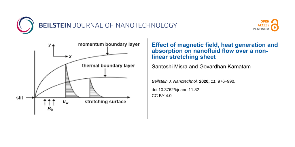
A two-dimensional, laminar, nonlinear steady-state boundary layer flow of a nanofluid across a permeable stretching surface was considered for study, as shown in Figure 1.
![[2190-4286-11-82-1]](/bjnano/content/figures/2190-4286-11-82-1.png?scale=2.0&max-width=1024&background=FFFFFF)
Figure 1: Two-dimensional coordinate system and fluid flow mechanism of a nanoparticle suspension.
Figure 1: Two-dimensional coordinate system and fluid flow mechanism of a nanoparticle suspension.
Figure 1 describes the stretching surface of a sheet taken along the x and y axes, normal to the surface. Fluid flow occurs when y ≥ 0, which is triggered when the sheet is stretched out of the slit occurring at the origin (when x = y = 0). The flow speed at any arbitrary point on the plate is assumed to be proportional to the power of its distance from the slit, considering boundary layer flow approximations at a distance of x units from the farthest edge. Considering a fixed origin, the sheet velocity is represented by uw(x) = axn, where n is the stretching parameter, a is the constant and x is the coordinate along the stretching surface.
The basic nanofluid governing equations in Cartesian form are given in the following where Tw and Cw represent the sheet temperature and the sheet nanoparticle fraction, respectively. The pressure and external forces are neglected and the nanoparticle fraction is assumed to be constant across the stretching surface. T∞ and C∞ denote ambient temperature and the associated nanoparticle fraction where Tw > T∞ and Cw > C∞. This physical model has significant applications in modern nanotechnology and thermal manufacturing in various industries.
Conservation of mass equation
![[2190-4286-11-82-i1]](/bjnano/content/inline/2190-4286-11-82-i1.svg?max-width=590&scale=1.18182)
Conservation of momentum equation (velocity)
![[2190-4286-11-82-i2]](/bjnano/content/inline/2190-4286-11-82-i2.svg?max-width=590&scale=1.18182)
Conservation of thermal energy equation (temperature)
![[2190-4286-11-82-i3]](/bjnano/content/inline/2190-4286-11-82-i3.svg?max-width=590&scale=1.18182)
Conservation of nanoparticle equation (concentration)
![[2190-4286-11-82-i4]](/bjnano/content/inline/2190-4286-11-82-i4.svg?max-width=590&scale=1.18182)
which is subjected to the following boundary conditions
![[2190-4286-11-82-i5]](/bjnano/content/inline/2190-4286-11-82-i5.svg?max-width=590&scale=1.18182)
![[2190-4286-11-82-i6]](/bjnano/content/inline/2190-4286-11-82-i6.svg?max-width=590&scale=1.18182)
and
![[2190-4286-11-82-i7]](/bjnano/content/inline/2190-4286-11-82-i7.svg?max-width=590&scale=1.18182)
αm denotes the thermal diffusivity, and τ denotes the ratio between effective heat capacities of the nanoparticle material and the base fluid. In Equations 1–4, u, and v denote the velocity components along x and y axes, respectively, ρf is the base fluid density, a is a positive constant, DB is the Brownian diffusion coefficient, DT denotes the thermodiffusion coefficient, c is the volumetric expansion coefficient, ρp is the particle density, σ denotes the nanofluid electrical conductivity, B0 denotes the magnetic induction, vw denotes the suction/injection velocity and Q0 (Q) denotes the heat generation (absorption) coefficient.
us in Equation 8 represents the slip velocity, given as
![[2190-4286-11-82-i8]](/bjnano/content/inline/2190-4286-11-82-i8.svg?max-width=590&scale=1.18182)
which is proportional to the local sheet stress, and l is the slip length constant.
The similarity transformations
The similarity transformations to solve the governing equations are as follows:
![[2190-4286-11-82-i9]](/bjnano/content/inline/2190-4286-11-82-i9.svg?max-width=590&scale=1.18182)
By substituting the similarity transformations in Equation 9 into the governing boundary layer Equations 1–4 they reduce to ordinary differential equations:
![[2190-4286-11-82-i10]](/bjnano/content/inline/2190-4286-11-82-i10.svg?max-width=590&scale=1.18182)
![[2190-4286-11-82-i11]](/bjnano/content/inline/2190-4286-11-82-i11.svg?max-width=590&scale=1.18182)
![[2190-4286-11-82-i12]](/bjnano/content/inline/2190-4286-11-82-i12.svg?max-width=590&scale=1.18182)
The transformed boundary conditions of Equation 5 and Equation 6, with regard to the similarity transformations in Equation 9, are:
![[2190-4286-11-82-i13]](/bjnano/content/inline/2190-4286-11-82-i13.svg?max-width=590&scale=1.18182)
![[2190-4286-11-82-i14]](/bjnano/content/inline/2190-4286-11-82-i14.svg?max-width=590&scale=1.18182)
The working rules for the boundary conditions are:
At y = 0: v = ±vw, where
![[Graphic 1]](/bjnano/content/inline/2190-4286-11-82-i19.svg?max-width=637&scale=1.18182)
at η = 0:
![[Graphic 2]](/bjnano/content/inline/2190-4286-11-82-i20.svg?max-width=637&scale=1.18182)
Therefore, f(η) = Fw where
![[Graphic 3]](/bjnano/content/inline/2190-4286-11-82-i21.svg?max-width=637&scale=1.18182)
at y = 0: u = uw + us where uw = axn, ![[Graphic 4]](/bjnano/content/inline/2190-4286-11-82-i22.svg?max-width=637&scale=1.18182) u = axnf´(η) where
u = axnf´(η) where
![[Graphic 5]](/bjnano/content/inline/2190-4286-11-82-i23.svg?max-width=637&scale=1.18182)
substituting the above values into u = uw + us we get:
![[Graphic 6]](/bjnano/content/inline/2190-4286-11-82-i24.svg?max-width=637&scale=1.18182)
Therefore, at η = 0: f = Fw, f´ = 1 + ξpf´´, θ = 1, ϕ = 1 when y → ∞: u → 0, T → T∞, C → C∞ henceforth as u → 0, f´(η) → 0, as T → T∞, θ(η) → 0, as C → C∞, ϕ(η) → 0
Therefore, at η → ∞: f´ → 0, θ → 0, ϕ → 0
The prime (´) denotes differentiation with respect to η, and the physical parameters involved in the equations are defined as follows:
![[2190-4286-11-82-i15]](/bjnano/content/inline/2190-4286-11-82-i15.svg?max-width=590&scale=1.18182)
The abbreviations used for the calculations are summarized in Table 1.
Table 1: Nomenclature for the basic nanofluid governing equations.
| Roman | Greek symbols | ||
| a | constant | αm | thermal diffusivity |
| n | nonlinear stretching parameter | ξp | slip parameter for liquids |
| C | nanoparticle volume fraction | υ | kinematic viscosity of the fluid |
| Cw | nanoparticle volume fraction at the sheet | τ |
torsion parameter defined by ![[Graphic 7]](/bjnano/content/inline/2190-4286-11-82-i25.svg?max-width=637&scale=1.0)
|
| C∞ | ambient nanoparticle volume fraction | ρcp | effective heat capacity of nanoparticles |
| Nt | thermophoresis parameter | ρcf | heat capacity of the fluid |
| Nb | Brownian motion parameter | η | similarity V |
| (x,y) | Cartesian coordinates | ϕ(η) | rescaled nanoparticle volume fraction |
| Tw | temperature at the sheet | θ(η) | dimensionless temperature |
| T∞ | ambient temperature | ρf | base fluid density |
| T | temperature | ρp | nanoparticle mass density |
| us | slip velocity | ||
| vw | suction/injection | ||
| DB | Brownian diffusion coefficient | ||
| DT | thermodiffusion coefficient | ||
| uw | velocity of the stretching sheet | ||
| M | magnetic field parameter | ||
| Q0/Q | heat generation/absorption coefficient | ||
| Le | Lewis number | ||
| Fw | suction/injection parameter | ||
| u, v | velocity components along x, y axes | ||
| σ | nanofluid electrical conductivity | ||
| B0 | magnetic induction | ||
| l | slip length constant | ||
| Pr | Prandtl number | ||
Solving a system of first-order differential equations
The nonlinear and coupled partial differential equations, represented by Equations 10–12, are solved by using the Adam’s predictor–corrector method which is the most efficient technique in numerical analysis used to solve distinctive problems related to heat transfer, fluid mechanics, and electrical systems. The first step involves reducing the nonlinear differential equations of third order in f and second order in θ and ϕ to a system of first-order differential equations, in order to simplify the problem as follows.
![[2190-4286-11-82-i16]](/bjnano/content/inline/2190-4286-11-82-i16.svg?max-width=590&scale=1.18182)
![[2190-4286-11-82-i17]](/bjnano/content/inline/2190-4286-11-82-i17.svg?max-width=590&scale=1.18182)
![[2190-4286-11-82-i18]](/bjnano/content/inline/2190-4286-11-82-i18.svg?max-width=590&scale=1.18182)
These equations were solved independently using a FORTRAN program which converts each one of them using different variables to first order as follows.
Equation 16 is represented as a system of equations for f as:
![[Graphic 8]](/bjnano/content/inline/2190-4286-11-82-i26.svg?max-width=637&scale=1.18182)
The boundary conditions with respect to η for f are:
![[Graphic 9]](/bjnano/content/inline/2190-4286-11-82-i27.svg?max-width=637&scale=1.18182)
We assume an initial guess value as α for y3, i.e., y3(0) = α. Hence, y1(0) = Fw, y2(0) = 1 + ξpα, y3(0) = α where α needs to be obtained by using Newton’s method to satisfy y2(η∞) → 0.
Equation 17 and Equation 18 are represented as follows by defining the system of equations for θ and ϕ:
![[Graphic 10]](/bjnano/content/inline/2190-4286-11-82-i28.svg?max-width=637&scale=1.18182)
The boundary conditions with respect to η for θ and ϕ are as follows:
![[Graphic 11]](/bjnano/content/inline/2190-4286-11-82-i29.svg?max-width=637&scale=1.18182)
The values of α and β, which are the unknowns with respect to θ and ϕ, are obtained by starting with an initial guess and then correcting the values using Newton’s method to satisfy the end conditions as follows:
![[Graphic 12]](/bjnano/content/inline/2190-4286-11-82-i30.svg?max-width=637&scale=1.18182)
The boundary value problem is converted to an initial value problem by reducing the equations, as shown above. The initial value problem is solved by using Adam’s predictor–corrector method and assigning an approximate initial value with step size h = 0.01 and η = 4 at the maximum value. The solution is obtained for different parameters used and convergence is achieved with a change in a single parameter. The criteria for convergence are the approximation up to three significant digits. The results derived through computation are plotted as graphs for a clear picture of the numerical problem (Table 2, Table 3).
Table 2: Computation of the streamwise velocity, temperature and concentration profiles for different values of the magnetic field parameter, M.
| η | M = 0.5 | M = 1.0 | M = 2.0 | M = 3.0 | ||||||||
| f´(η) | θ(η) | ϕ(η) | f´(η) | θ(η) | ϕ(η) | f´(η) | θ(η) | ϕ(η) | f´(η) | θ(η) | ϕ(η) | |
| 0 | 0.468 | 1 | 1 | 0.428 | 1 | 1 | 0.375 | 1 | 1 | 0.339 | 1 | 1 |
| 0.2 | 0.373 | 0.935 | 0.714 | 0.328 | 0.94 | 0.726 | 0.268 | 0.946 | 0.74 | 0.23 | 0.949 | 0.749 |
| 0.4 | 0.298 | 0.855 | 0.51 | 0.252 | 0.866 | 0.528 | 0.193 | 0.881 | 0.549 | 0.156 | 0.889 | 0.563 |
| 0.6 | 0.238 | 0.766 | 0.374 | 0.193 | 0.784 | 0.392 | 0.138 | 0.808 | 0.415 | 0.106 | 0.823 | 0.429 |
| 0.8 | 0.19 | 0.672 | 0.286 | 0.149 | 0.699 | 0.302 | 0.099 | 0.732 | 0.323 | 0.072 | 0.753 | 0.335 |
| 1.0 | 0.152 | 0.581 | 0.229 | 0.114 | 0.614 | 0.242 | 0.071 | 0.656 | 0.259 | 0.049 | 0.681 | 0.269 |
| 1.2 | 0.122 | 0.494 | 0.189 | 0.088 | 0.532 | 0.2 | 0.051 | 0.581 | 0.214 | 0.033 | 0.611 | 0.221 |
| 1.4 | 0.098 | 0.414 | 0.159 | 0.068 | 0.456 | 0.17 | 0.037 | 0.51 | 0.18 | 0.023 | 0.543 | 0.186 |
| 1.6 | 0.078 | 0.342 | 0.136 | 0.052 | 0.386 | 0.145 | 0.027 | 0.443 | 0.155 | 0.015 | 0.478 | 0.159 |
| 1.8 | 0.062 | 0.279 | 0.115 | 0.04 | 0.323 | 0.125 | 0.019 | 0.38 | 0.134 | 0.01 | 0.417 | 0.137 |
| 2.0 | 0.049 | 0.225 | 0.097 | 0.031 | 0.267 | 0.107 | 0.014 | 0.323 | 0.115 | 0.007 | 0.359 | 0.119 |
| 2.2 | 0.039 | 0.179 | 0.08 | 0.023 | 0.218 | 0.09 | 0.01 | 0.272 | 0.099 | 0.005 | 0.306 | 0.102 |
| 2.4 | 0.031 | 0.14 | 0.066 | 0.018 | 0.175 | 0.075 | 0.007 | 0.225 | 0.084 | 0.003 | 0.257 | 0.087 |
| 2.6 | 0.024 | 0.107 | 0.053 | 0.014 | 0.138 | 0.062 | 0.005 | 0.183 | 0.071 | 0.002 | 0.213 | 0.074 |
| 2.8 | 0.018 | 0.081 | 0.041 | 0.01 | 0.107 | 0.049 | 0.004 | 0.146 | 0.058 | 0.001 | 0.172 | 0.061 |
| 3.0 | 0.014 | 0.059 | 0.031 | 0.007 | 0.08 | 0.038 | 0.003 | 0.113 | 0.046 | 0.001 | 0.135 | 0.049 |
| 3.2 | 0.01 | 0.042 | 0.022 | 0.005 | 0.058 | 0.028 | 0.002 | 0.084 | 0.035 | 0.001 | 0.102 | 0.038 |
| 3.4 | 0.007 | 0.027 | 0.015 | 0.004 | 0.039 | 0.02 | 0.001 | 0.058 | 0.025 | 0 | 0.072 | 0.028 |
| 3.6 | 0.004 | 0.016 | 0.009 | 0.002 | 0.024 | 0.012 | 0.001 | 0.036 | 0.016 | 0 | 0.045 | 0.018 |
| 3.8 | 0.002 | 0.007 | 0.004 | 0.001 | 0.011 | 0.006 | 0 | 0.017 | 0.008 | 0 | 0.021 | 0.009 |
| 4.0 | 0 | 0 | 0 | 0 | 0 | 0 | 0 | 0 | 0 | 0 | 0 | 0 |
Table 3: Computation of streamwise velocity, temperature and concentration profiles for different values of the heat generation/absorption coefficient, Q.
| η | Q = 0.0 | Q = 0.2 | Q = 0.3 | ||||||
| f´(η) | θ(η) | ϕ(η) | f´(η) | θ(η) | ϕ(η) | f´(η) | θ(η) | ϕ(η) | |
| 0 | 0.524 | 1 | 1 | 0.524 | 1 | 1 | 0.524 | 1 | 1 |
| 0.2 | 0.437 | 0.928 | 0.697 | 0.437 | 0.95 | 0.682 | 0.437 | 1.028 | 0.627 |
| 0.4 | 0.365 | 0.839 | 0.485 | 0.365 | 0.88 | 0.462 | 0.365 | 1.035 | 0.367 |
| 0.6 | 0.306 | 0.738 | 0.349 | 0.306 | 0.794 | 0.322 | 0.306 | 1.018 | 0.208 |
| 0.8 | 0.256 | 0.634 | 0.263 | 0.256 | 0.701 | 0.238 | 0.256 | 0.977 | 0.124 |
| 1.0 | 0.214 | 0.533 | 0.209 | 0.214 | 0.605 | 0.189 | 0.214 | 0.918 | 0.088 |
| 1.2 | 0.179 | 0.439 | 0.172 | 0.179 | 0.513 | 0.158 | 0.179 | 0.845 | 0.076 |
| 1.4 | 0.149 | 0.355 | 0.143 | 0.149 | 0.427 | 0.135 | 0.149 | 0.764 | 0.076 |
| 1.6 | 0.124 | 0.283 | 0.119 | 0.124 | 0.35 | 0.117 | 0.124 | 0.678 | 0.079 |
| 1.8 | 0.103 | 0.221 | 0.099 | 0.103 | 0.281 | 0.1 | 0.103 | 0.591 | 0.082 |
| 2.0 | 0.085 | 0.17 | 0.08 | 0.085 | 0.223 | 0.085 | 0.085 | 0.506 | 0.082 |
| 2.2 | 0.069 | 0.129 | 0.064 | 0.069 | 0.174 | 0.07 | 0.069 | 0.424 | 0.079 |
| 2.4 | 0.056 | 0.096 | 0.05 | 0.056 | 0.133 | 0.057 | 0.056 | 0.348 | 0.074 |
| 2.6 | 0.045 | 0.071 | 0.038 | 0.045 | 0.1 | 0.045 | 0.045 | 0.278 | 0.067 |
| 2.8 | 0.035 | 0.051 | 0.028 | 0.035 | 0.073 | 0.035 | 0.035 | 0.216 | 0.058 |
| 3.0 | 0.027 | 0.036 | 0.021 | 0.027 | 0.052 | 0.026 | 0.027 | 0.162 | 0.048 |
| 3.2 | 0.02 | 0.024 | 0.014 | 0.02 | 0.036 | 0.018 | 0.02 | 0.115 | 0.037 |
| 3.4 | 0.014 | 0.015 | 0.009 | 0.014 | 0.023 | 0.012 | 0.014 | 0.076 | 0.027 |
| 3.6 | 0.008 | 0.009 | 0.005 | 0.008 | 0.013 | 0.007 | 0.008 | 0.045 | 0.017 |
| 3.8 | 0.004 | 0.004 | 0.002 | 0.004 | 0.006 | 0.003 | 0.004 | 0.019 | 0.008 |
| 4.0 | 0 | 0 | 0 | 0 | 0 | 0 | 0 | 0 | 0 |
Results and Discussion
To provide physical insight into the flow problem, numerical computations involving various parameters and their influence on the dimensionless velocity, temperature and nanoparticle concentration of fluid flow have been represented graphically as follows.
Impact of ξ on f´(η)
Figure 2 illustrates the influence of the slip parameter, ξ, on the velocity gradient which decreases with an increase in the value of ξ, converging to zero at the end of the boundary layer, thus causing a reduction in its thickness for nanofluids. This is due to the fact that an increase in the slip parameter causes a reduction in the skin friction at the surface acting between the stretching sheet and the fluid flow, thus drastically decreasing the velocity gradient.
![[2190-4286-11-82-2]](/bjnano/content/figures/2190-4286-11-82-2.png?scale=2.0&max-width=1024&background=FFFFFF)
Figure 2: Influence of the slip parameter for liquids ξ on the streamwise velocity component f´(η) when n = 2.0, M = 0.0, Q = 0.0, Pr = 2.0, Nb = Nt = 0.5, Le = 5.0, and Fw = 0.2.
Figure 2: Influence of the slip parameter for liquids ξ on the streamwise velocity component f´(η) when n = 2...
Impact of ξ on θ(η)
The temperature variation component, θ(η), increases with an increase in the slip parameter, ξ, which further leads to an increase in the fluid temperature, thus intensifying the thermal boundary layer thickness (Figure 3). An increase in the slip parameter causes friction at the surface which, in turn, generates a frictional force allowing more fluid to flow passed the stretching sheet, causing an increase in the temperature gradient and reducing the velocity of the fluid.
![[2190-4286-11-82-3]](/bjnano/content/figures/2190-4286-11-82-3.png?scale=2.0&max-width=1024&background=FFFFFF)
Figure 3: Influence of the slip parameter for liquids ξ on the temperature distribution θ(η) when n = 2.0, M = 0.0, Q = 0.0, Pr = 2.0, Nb = Nt = 0.5, Le = 5.0, and Fw = 0.2.
Figure 3: Influence of the slip parameter for liquids ξ on the temperature distribution θ(η) when n = 2.0, M ...
Impact of ξ on ϕ(η)
The nanoparticle concentration distribution, ϕ(η), increases with an increase in the slip parameter, ξ, at a given constant surface temperature. An increase in the slip parameter causes friction at the surface which, in turn, generates a frictional force allowing more fluid to flow passed the stretching sheet. This causes an increase in concentration distribution of the fluid as shown in Figure 4, which ultimately reduces the fluid velocity.
![[2190-4286-11-82-4]](/bjnano/content/figures/2190-4286-11-82-4.png?scale=2.0&max-width=1024&background=FFFFFF)
Figure 4: Influence of the slip parameter for liquids ξ on the concentration distribution ϕ(η) when n = 2.0, M = 0.0, Q = 0.0, Pr = 2.0, Nb = Nt = 0.5, Le = 5.0, and Fw = 0.2.
Figure 4: Influence of the slip parameter for liquids ξ on the concentration distribution ϕ(η) when n = 2.0, M...
Impact of n on f´(η)
The nonlinear stretching parameter, n, has a significant influence on the fluid flow velocity component, f´(η). Figure 5 shows that with an increase in n, the velocity gradient decreases, thus depleting the thickness of the momentum boundary layer. This is due to the fact that, with the sheet being stretched, there is a retarding force in the fluid in which the fluid particles have severe impact on the velocity component leading to its reduction as we move away from the boundary layer.
![[2190-4286-11-82-5]](/bjnano/content/figures/2190-4286-11-82-5.png?scale=2.0&max-width=1024&background=FFFFFF)
Figure 5: Influence of the stretching parameter n on the streamwise velocity component f´(η) when ξ = M = Q = 0.0, Pr = 2.0, Nb = Nt = 0.5, Le = 5.0, and Fw = 0.2.
Figure 5: Influence of the stretching parameter n on the streamwise velocity component f´(η) when ξ = M = Q =...
Impact of n on θ(η)
With an increase in the stretching parameter, n, the temperature gradient, θ(η), increases leading to an increase in the thermal boundary layer thickness. As the value of the stretching parameter increases, the convection process in the particles of the fluid flow intensifies, thus leading to a rapid increase in the temperature gradient which, in turn, is responsible for an increase in the thermal boundary layer thickness (Figure 6).
![[2190-4286-11-82-6]](/bjnano/content/figures/2190-4286-11-82-6.png?scale=2.0&max-width=1024&background=FFFFFF)
Figure 6: Influence of the stretching parameter n on the temperature distribution θ(η) when ξ = 1.0, M = Q = 0.0, Pr = 2.0, Nb = Nt = 0.5, Le = 5.0, and Fw = 0.2 (due to the boundary condition, the value of ξ is changed).
Figure 6: Influence of the stretching parameter n on the temperature distribution θ(η) when ξ = 1.0, M = Q = ...
Impact of n on ϕ(η)
With an increase in the stretching parameter, n, the concentration profile of the fluid, ϕ(η), increases slightly but the effect observed is not significant, which is noticed at higher values of n. At lower values of the stretching parameter, there is a negligible change in the fluid concentration of the fluid, which is independent of stretch. On the other hand, there is a significant increase in the stretching parameter at extremely high values that does not seem to affect the fluid particle concentration (Figure 7).
![[2190-4286-11-82-7]](/bjnano/content/figures/2190-4286-11-82-7.png?scale=2.0&max-width=1024&background=FFFFFF)
Figure 7: Influence of the stretching parameter n on the concentration distribution ϕ(η) when ξ = 1.0, M = Q = 0.0, Pr = 2.0, Nb = Nt = 0.5, Le = 5.0, and Fw = 0.2 (due to the boundary condition, the value of ξ is changed).
Figure 7: Influence of the stretching parameter n on the concentration distribution ϕ(η) when ξ = 1.0, M = Q ...
Impact of Nb on θ(η)
The Brownian motion parameter, Nb, has a remarkable effect on the temperature gradient, θ(η). When Nb increases, it leads to an increase in θ(η) which causes an increase in the thermal boundary layer thickness of the fluid flow. Higher Brownian motion is responsible for fast movement of fluid particles which, in turn, induces either an increase in acceleration or random acceleration levels resulting in additional energy among particles and, consequently, an increase in the temperature gradient and thermal boundary layer thickness (Figure 8).
![[2190-4286-11-82-8]](/bjnano/content/figures/2190-4286-11-82-8.png?scale=2.0&max-width=1024&background=FFFFFF)
Figure 8: Influence of the Brownian motion parameter Nb on the temperature distribution, θ(η) when n = 2.0, ξ = 1.0, M = Q = 0.0, Pr = 2.0, Nt = 0.5, Le = 5.0, and Fw = 0.2.
Figure 8: Influence of the Brownian motion parameter Nb on the temperature distribution, θ(η) when n = 2.0, ξ...
Impact of Nb on ϕ(η)
An increase in the Brownian motion parameter, Nb, results in a decrease in the concentration gradient of the fluid, ϕ(η), due to the fact that the particles move from a high to a low concentration region. As the movement of the fluid particles intensifies with an increase in the Brownian motion, the particles start moving rapidly from regions of higher to regions of lower concentration since the random acceleration decreases the concentration gradient of the fluid flow (Figure 9).
![[2190-4286-11-82-9]](/bjnano/content/figures/2190-4286-11-82-9.png?scale=2.0&max-width=1024&background=FFFFFF)
Figure 9: Influence of the Brownian motion parameter Nb on the concentration distribution ϕ(η) when n = 2.0, ξ = 1.0, M = Q = 0.0, Pr = 2.0, Nt = 0.5, Le = 5.0, and Fw = 0.2.
Figure 9: Influence of the Brownian motion parameter Nb on the concentration distribution ϕ(η) when n = 2.0, ...
Impact of Nt on θ(η)
With an increase in the thermophoresis parameter, Nt, the temperature gradient of the fluid, θ(η), also increases leading to an enhancement in the thermal boundary layer thickness. Due to the presence of a temperature gradient, different particles of the fluid exhibit different responses to the change in the thermophoresis parameter. As Nt increases, the particles start moving rapidly which causes an elevation in the kinetic energy of the system, resulting in an increase in the temperature distribution and in the boundary layer thickness (Figure 10).
![[2190-4286-11-82-10]](/bjnano/content/figures/2190-4286-11-82-10.png?scale=2.0&max-width=1024&background=FFFFFF)
Figure 10: Influence of the thermophoresis parameter Nt on the temperature distribution θ(η) when n = 2.0, ξ = 1.0, M = Q = 0.0, Pr = 2.0, Nb = 0.5, Le = 5.0, and Fw = 0.2.
Figure 10: Influence of the thermophoresis parameter Nt on the temperature distribution θ(η) when n = 2.0, ξ =...
Impact of Nt on ϕ(η)
A small increase in thermophoresis parameter, Nt, causes a massive increase in the concentration distribution of the fluid flow, ϕ(η), which converges to zero at the boundary layer. A small change in the thermophoresis parameter leads to rapid motion in the fluid particles creating excess heat energy and leading to a massive increase in the concentration distribution. Therefore, Figure 11 shows a significant increase in the concentration distribution with a very slight increase in the value of Nt.
![[2190-4286-11-82-11]](/bjnano/content/figures/2190-4286-11-82-11.png?scale=2.0&max-width=1024&background=FFFFFF)
Figure 11: Influence of the thermophoresis parameter Nt on the concentration distribution ϕ(η) when n = 2.0, ξ = 1.0, M = Q = 0.0, Pr = 2.0, Nb = 0.5, Le = 5.0, and Fw = 0.2.
Figure 11: Influence of the thermophoresis parameter Nt on the concentration distribution ϕ(η) when n = 2.0, ξ...
Impact of M on f´(η)
An increase in the magnetic parameter, M, leads to a decrease in the streamwise velocity component, f´(η), which, in turn, reduces the velocity boundary layer thickness. The external magnetic field has a massive effect on the velocity profile of an electrically conducting fluid, which causes a considerable amount of resistance to its motion and a driving force, called the Lorentz force, which reduces the fluid velocity (Figure 12).
![[2190-4286-11-82-12]](/bjnano/content/figures/2190-4286-11-82-12.png?scale=2.0&max-width=1024&background=FFFFFF)
Figure 12: Influence of the magnetic parameter M on the streamwise velocity component f´(η) when n = 2.0, Pr = 2.0, Nb = Nt = 0.5, Q = 0.0, Le = 5.0, ξ = 1.0, and Fw = 0.2.
Figure 12: Influence of the magnetic parameter M on the streamwise velocity component f´(η) when n = 2.0, Pr =...
Impact of M on θ(η)
With an increase in the magnetic parameter, M, and, consequently, of the fluid resistance, the fluid temperature profile, θ(η), increases and so does the thickness of the thermal boundary layer. This is due to the fact that with an external magnetic field being employed, the temperature of the fluid increases, resulting in the rapid movement of the fluid particles which increases both the thermal energy and the boundary layer thickness and reduces the heat transfer from the sheet (Figure 13).
![[2190-4286-11-82-13]](/bjnano/content/figures/2190-4286-11-82-13.png?scale=2.0&max-width=1024&background=FFFFFF)
Figure 13: Influence of the magnetic parameter M on the temperature distribution θ(η) when n = 2.0, Pr = 2.0, Nb = Nt = 0.5, Q = 0.0, Le = 5.0, ξ = 1.0, and Fw = 0.2.
Figure 13: Influence of the magnetic parameter M on the temperature distribution θ(η) when n = 2.0, Pr = 2.0, ...
Impact of M on ϕ(η)
An increase in the magnetic parameter, M, does not have much influence on the concentration distribution, ϕ(η), which is depicted in Figure 14. Even though there is a minimal increasing trend observed, the flow seems invariable. Since the concentration gradient of the fluid flow is not significantly modified by the external magnetic field applied, there is not much of a change in particle motion upon an increase in M values (Figure 14).
![[2190-4286-11-82-14]](/bjnano/content/figures/2190-4286-11-82-14.png?scale=2.0&max-width=1024&background=FFFFFF)
Figure 14: Influence of magnetic parameter M on the concentration distribution ϕ(η) when n = 2.0, Pr = 2.0, Nb = Nt = 0.5, Q = 0.0, Le = 5.0, ξ = 1.0, and Fw = 0.2.
Figure 14: Influence of magnetic parameter M on the concentration distribution ϕ(η) when n = 2.0, Pr = 2.0, Nb...
Impact of Q on f´(η)
The effect of the heat generation/absorption coefficient, Q, on the streamwise velocity component, f´(η), is negligible and, therefore, it does not affect the fluid flow velocity. The value of the heat generation/absorption coefficient being positive demonstrates that the heat generated does not have much impact on the velocity gradient of the fluid as the fluid particles move at the same velocity (Figure 15).
![[2190-4286-11-82-15]](/bjnano/content/figures/2190-4286-11-82-15.png?scale=2.0&max-width=1024&background=FFFFFF)
Figure 15: Influence of the heat generation/absorption coefficient Q on the streamwise velocity component f´(η) when n = 2.0, Pr = 2.0, Nb = Nt = 0.5, M = 0.0, Le = 5.0, Fw = 0.2, and ξ = 1.0.
Figure 15: Influence of the heat generation/absorption coefficient Q on the streamwise velocity component f´(η...
Impact of Q on θ(η)
The heat generation/absorption coefficient, Q, has a considerable effect on the dimensionless temperature profile of the fluid, θ(η), which increases with an increase in the value of Q as shown in Figure 16. An increase in the fluid temperature increases the thermal boundary layer thickness. The presence of an external heat source has a significant impact on the temperature gradient of the fluid, resulting in an increase in both the temperature distribution and thermal state of the fluid. With a massive amount of heat energy generated among fluid particles, the thermal boundary layer thickness increases to a larger extent (Figure 16).
![[2190-4286-11-82-16]](/bjnano/content/figures/2190-4286-11-82-16.png?scale=2.0&max-width=1024&background=FFFFFF)
Figure 16: Influence of the heat generation/absorption coefficient Q on the temperature distribution θ(η) when n = 2.0, Pr = 2.0, Nb = Nt = 0.5, M = 0.0, Le = 5.0, Fw = 0.2, and ξ = 1.0.
Figure 16: Influence of the heat generation/absorption coefficient Q on the temperature distribution θ(η) when ...
Impact of Q on ϕ(η)
The heat generation/absorption coefficient, Q, does not have much of an effect on the concentration distribution, ϕ(η), as the concentration of the fluid remains unaltered with the change of heat in the fluid. The heat generation coefficient is responsible for changing the heat gradient of the fluid flow, which has a negligible influence on the concentration levels of the fluid particles (Figure 17).
![[2190-4286-11-82-17]](/bjnano/content/figures/2190-4286-11-82-17.png?scale=2.0&max-width=1024&background=FFFFFF)
Figure 17: Influence of the heat generation/absorption coefficient Q on the concentration distribution ϕ(η) when n = 2.0, Pr = 2.0, Nb = Nt = 0.5, M = 0.0, Le = 5.0, Fw = 0.2, and ξ = 1.0.
Figure 17: Influence of the heat generation/absorption coefficient Q on the concentration distribution ϕ(η) wh...
Conclusion
In this work, it was found that an increase in the slip parameter, ξ, significantly reduces the fluid streamwise velocity gradient which, in turn, reduces the boundary layer thickness. On the other hand, an increase in ξ causes an increase in both the temperature θ(η) and concentration gradients ϕ(η). It was also found that an increase in the stretching parameter n reduces the velocity gradient, thus, depleting the boundary layer; however, the temperature and nanoparticle concentration of the flow were found to increase. An increase in the Brownian motion parameter, Nb, was found to increase the temperature gradient but reduce the concentration of the fluid, whereas the increase in the thermophoresis parameter, Nt, was found to increase both θ(η) and ϕ(η). The external magnetic field was found to have an enormous influence on the velocity gradient of the fluid which decreases with an increase in M due to a drag-like force, or resistance, that is developed by the fluid. Another observation was that the temperature gradient considerably increases with an increase in M, thus enhancing the thermal boundary layer thickness of the fluid as the external magnetic field does not have much of an effect on the concentration gradient. It was also shown that an increase in the heat generation/absorption coefficient, Q, results in a significant increase in the temperature profile without changing the velocity or the concentration of the fluid. With Q being positive, there is heat generation across the flow, which enhances the thermal boundary layer thickness.
References
-
Sakiadis, B. C. AIChE J. 1961, 7, 26–28. doi:10.1002/aic.690070108
Return to citation in text: [1] -
Sakiadis, B. C. AIChE J. 1961, 7, 221–225. doi:10.1002/aic.690070211
Return to citation in text: [1] -
Crane, L. J. Z. Angew. Math. Phys. 1970, 21, 645–647. doi:10.1007/bf01587695
Return to citation in text: [1] -
Chamhka, A. J.; Issa, C. Int. J. Numer. Methods Heat Fluid Flow 2000, 10, 432–449. doi:10.1108/09615530010327404
Return to citation in text: [1] -
Anderson, J. D., Jr. Explicit Finite Difference Methods: Some Selected Applications to Inviscid and Viscous Flows. Computational Fluid Dynamics; Springer-Verlag: Berlin, Heidelberg, Germany, 2009; pp 127–149. doi:10.1007/978-3-540-85056-4_7
Return to citation in text: [1] -
Khan, W. A.; Pop, I. Int. J. Heat Mass Transfer 2010, 53, 2477–2483. doi:10.1016/j.ijheatmasstransfer.2010.01.032
Return to citation in text: [1] -
Rana, P.; Bhargava, R. Commun. Nonlinear Sci. Numer. Simul. 2012, 17, 212–226. doi:10.1016/j.cnsns.2011.05.009
Return to citation in text: [1] -
Das, K. J. Egypt. Math. Soc. 2015, 23, 451–456. doi:10.1016/j.joems.2014.06.014
Return to citation in text: [1] -
Hayat, T.; Imtiaz, M.; Alsaedi, A. Appl. Math. Mech. (Engl. Ed.) 2015, 36, 1513–1526. doi:10.1007/s10483-015-1999-7
Return to citation in text: [1] -
Besthapu, P.; Bandari, S. J. Appl. Math. Phys. 2015, 3, 1580–1593. doi:10.4236/jamp.2015.312182
Return to citation in text: [1] -
Abdul Gaffar, S.; Ramachandra Prasad, V.; Keshava Reddy, E.; Anwar Bég, O. Ain Shams Eng. J. 2015, 6, 1009–1030. doi:10.1016/j.asej.2015.02.014
Return to citation in text: [1] -
Dogonchi, A. S.; Ganji, D. D. J. Mol. Liq. 2016, 223, 521–527. doi:10.1016/j.molliq.2016.08.090
Return to citation in text: [1] -
Farooq, M.; Anjum, A.; Hayat, T.; Alsaedi, A. J. Mol. Liq. 2016, 224, 1341–1347. doi:10.1016/j.molliq.2016.10.123
Return to citation in text: [1] -
Qayyum, S.; Hayat, T.; Alsaedi, A. Results Phys. 2017, 7, 2752–2761. doi:10.1016/j.rinp.2017.07.043
Return to citation in text: [1] -
Sreekala, B.; Janardhan, K.; Ramya, D.; Shravani, I. Global J. Pure Appl. Math. 2017, 13, 4927–4941.
Return to citation in text: [1] -
Rashid, I.; Ul Haq, R.; Al-Mdallal, Q. M. Phys. E (Amsterdam, Neth.) 2017, 89, 33–42. doi:10.1016/j.physe.2017.01.029
Return to citation in text: [1] -
Ahmad, R.; Mustafa, M.; Turkyilmazoglu, M. Int. J. Heat Mass Transfer 2017, 111, 827–835. doi:10.1016/j.ijheatmasstransfer.2017.04.046
Return to citation in text: [1] -
Seth, G. S.; Bhattacharyya, A.; Kumar, R.; Chamkha, A. J. Phys. Fluids 2018, 30, 122003. doi:10.1063/1.5054099
Return to citation in text: [1] -
Soomro, F. A.; Ul Haq, R.; Al-Mdallal, Q. M.; Zhang, Q. Results Phys. 2018, 8, 404–414. doi:10.1016/j.rinp.2017.12.037
Return to citation in text: [1] -
Soomro, F. A.; Usman, M.; Ul Haq, R.; Wang, W. Int. J. Heat Mass Transfer 2018, 126, 1034–1042. doi:10.1016/j.ijheatmasstransfer.2018.05.099
Return to citation in text: [1] -
Farooq, A.; Ali, R.; Benim, A. C. Phys. A (Amsterdam, Neth.) 2018, 503, 345–354. doi:10.1016/j.physa.2018.02.204
Return to citation in text: [1] -
Irfan, M.; Farooq, M. A.; Iqra, T. Front. Phys. 2019, 7, 186. doi:10.3389/fphy.2019.00186
Return to citation in text: [1] -
Pal, D.; Mondal, S.; Mondal, H. Int. J. Ambient Energy 2019, 1–15. doi:10.1080/01430750.2019.1614984
Return to citation in text: [1] -
Shah, Z.; Babazadeh, H.; Kumam, P.; Shafee, A.; Thounthong, P. Front. Phys. 2019, 7, 164. doi:10.3389/fphy.2019.00164
Return to citation in text: [1] -
Yousif, M. A.; Ismael, H. F.; Abbas, T.; Ellahi, R. Heat Transfer Res. 2019, 50, 649–658. doi:10.1615/heattransres.2018025568
Return to citation in text: [1]
| 19. | Soomro, F. A.; Ul Haq, R.; Al-Mdallal, Q. M.; Zhang, Q. Results Phys. 2018, 8, 404–414. doi:10.1016/j.rinp.2017.12.037 |
| 20. | Soomro, F. A.; Usman, M.; Ul Haq, R.; Wang, W. Int. J. Heat Mass Transfer 2018, 126, 1034–1042. doi:10.1016/j.ijheatmasstransfer.2018.05.099 |
| 17. | Ahmad, R.; Mustafa, M.; Turkyilmazoglu, M. Int. J. Heat Mass Transfer 2017, 111, 827–835. doi:10.1016/j.ijheatmasstransfer.2017.04.046 |
| 18. | Seth, G. S.; Bhattacharyya, A.; Kumar, R.; Chamkha, A. J. Phys. Fluids 2018, 30, 122003. doi:10.1063/1.5054099 |
| 5. | Anderson, J. D., Jr. Explicit Finite Difference Methods: Some Selected Applications to Inviscid and Viscous Flows. Computational Fluid Dynamics; Springer-Verlag: Berlin, Heidelberg, Germany, 2009; pp 127–149. doi:10.1007/978-3-540-85056-4_7 |
| 15. | Sreekala, B.; Janardhan, K.; Ramya, D.; Shravani, I. Global J. Pure Appl. Math. 2017, 13, 4927–4941. |
| 4. | Chamhka, A. J.; Issa, C. Int. J. Numer. Methods Heat Fluid Flow 2000, 10, 432–449. doi:10.1108/09615530010327404 |
| 16. | Rashid, I.; Ul Haq, R.; Al-Mdallal, Q. M. Phys. E (Amsterdam, Neth.) 2017, 89, 33–42. doi:10.1016/j.physe.2017.01.029 |
| 13. | Farooq, M.; Anjum, A.; Hayat, T.; Alsaedi, A. J. Mol. Liq. 2016, 224, 1341–1347. doi:10.1016/j.molliq.2016.10.123 |
| 25. | Yousif, M. A.; Ismael, H. F.; Abbas, T.; Ellahi, R. Heat Transfer Res. 2019, 50, 649–658. doi:10.1615/heattransres.2018025568 |
| 14. | Qayyum, S.; Hayat, T.; Alsaedi, A. Results Phys. 2017, 7, 2752–2761. doi:10.1016/j.rinp.2017.07.043 |
| 9. | Hayat, T.; Imtiaz, M.; Alsaedi, A. Appl. Math. Mech. (Engl. Ed.) 2015, 36, 1513–1526. doi:10.1007/s10483-015-1999-7 |
| 11. | Abdul Gaffar, S.; Ramachandra Prasad, V.; Keshava Reddy, E.; Anwar Bég, O. Ain Shams Eng. J. 2015, 6, 1009–1030. doi:10.1016/j.asej.2015.02.014 |
| 23. | Pal, D.; Mondal, S.; Mondal, H. Int. J. Ambient Energy 2019, 1–15. doi:10.1080/01430750.2019.1614984 |
| 8. | Das, K. J. Egypt. Math. Soc. 2015, 23, 451–456. doi:10.1016/j.joems.2014.06.014 |
| 12. | Dogonchi, A. S.; Ganji, D. D. J. Mol. Liq. 2016, 223, 521–527. doi:10.1016/j.molliq.2016.08.090 |
| 24. | Shah, Z.; Babazadeh, H.; Kumam, P.; Shafee, A.; Thounthong, P. Front. Phys. 2019, 7, 164. doi:10.3389/fphy.2019.00164 |
| 7. | Rana, P.; Bhargava, R. Commun. Nonlinear Sci. Numer. Simul. 2012, 17, 212–226. doi:10.1016/j.cnsns.2011.05.009 |
| 21. | Farooq, A.; Ali, R.; Benim, A. C. Phys. A (Amsterdam, Neth.) 2018, 503, 345–354. doi:10.1016/j.physa.2018.02.204 |
| 6. | Khan, W. A.; Pop, I. Int. J. Heat Mass Transfer 2010, 53, 2477–2483. doi:10.1016/j.ijheatmasstransfer.2010.01.032 |
| 10. | Besthapu, P.; Bandari, S. J. Appl. Math. Phys. 2015, 3, 1580–1593. doi:10.4236/jamp.2015.312182 |
| 22. | Irfan, M.; Farooq, M. A.; Iqra, T. Front. Phys. 2019, 7, 186. doi:10.3389/fphy.2019.00186 |
© 2020 Misra and Kamatam; licensee Beilstein-Institut.
This is an Open Access article under the terms of the Creative Commons Attribution License (http://creativecommons.org/licenses/by/4.0). Please note that the reuse, redistribution and reproduction in particular requires that the authors and source are credited.
The license is subject to the Beilstein Journal of Nanotechnology terms and conditions: (https://www.beilstein-journals.org/bjnano)