Abstract
In this paper, we derive and present quantitative expressions governing the performance of single and multifrequency Kelvin probe force microscopy (KPFM) techniques in both air and water. Metrics such as minimum detectable contact potential difference, minimum required AC bias, and signal-to-noise ratio are compared and contrasted both off resonance and utilizing the first two eigenmodes of the cantilever. These comparisons allow the reader to quickly and quantitatively identify the parameters for the best performance for a given KPFM-based experiment in a given environment. Furthermore, we apply these performance metrics in the identification of KPFM-based modes that are most suitable for operation in liquid environments where bias application can lead to unwanted electrochemical reactions. We conclude that open-loop multifrequency KPFM modes operated with the first harmonic of the electrostatic response on the first eigenmode offer the best performance in liquid environments whilst needing the smallest AC bias for operation.
Introduction
Atomic force microscopy (AFM) is an enabling technique for the nanoscale mapping of topography and surface properties of interfaces in a wide range of environments [1]. Kelvin probe force microscopy (KPFM) utilizes the application of a bias and a conductive probe to map the local electrical properties of an interface at the nanoscale [2], allowing for the determination of the local contact potential difference (CPD) between the probe and the sample. This, in turn, allows the work function of the sample to be measured if the work function of the probe is known and vice versa. The mapping of local electrical properties of the interface is essential to further our understanding of corrosion, sensing, solar cells, energy storage devices, and bioelectric interfaces [3-8]. Since its first application in 1991 [2], there have been significant developments in the field of KPFM [6,9,10] with significant advances in both temporal [11-14] and spatial resolution [13,15-19]. These advances have enabled investigations mapping light-induced surface potential dynamics [20], ferroelectric domains [19], individual quantum dots [21,22], and even submolecular charge distributions [23-27]. These applications demonstrate that KPFM is capable of atomic-scale spatial resolution and nanosecond time resolution under specific conditions.
KPFM-based techniques can largely be classified as either “open loop” (OL) or “closed loop” (CL). CL techniques employ a feedback loop to apply a bias to compensate for the electrostatic force (or force gradient) between the tip and sample. CL techniques are more common than OL techniques due to the ease of implementation, wide-scale availability, and direct measurement of the apparent CPD. OL techniques, by contrast, are feedback-free and can be used to determine the CPD without the need to apply a DC bias [28,29]. OL techniques are increasingly being adopted to enable the mapping of voltage-sensitive materials [30-32], to enable investigations of fast electrodynamic processes [11-14] and to enable measurements in liquid environments (where bias application could lead to stray currents and unwanted electrochemical reactions) [9,33-35]. OL techniques avoid the limitations and artefacts that can arise when using a feedback loop, for example, bandwidth limitations due to the time constant of the feedback loop [29], increased noise [36,37], and electrical crosstalk [38,39]. Whilst the application of DC bias is not required for OL operation it can still be utilized to allow CPD to be determined via bias sweeps [28,40] or to investigate gate-dependent potential profiles of interfaces [22,41,42]. There are a wide range of OL KPFM techniques beyond those examined in this paper, including pump-probe KPFM [13,20,43], time-resolved KPFM [11,12,44-47], fast free force recovery KPFM (G-Mode) [14,48-50], intermodulation electrostatic force microscopy (EFM) [42,51], and PeakForce tapping KPFM [52].
The fundamental detection sensitivity to electrostatic forces in KPFM is generally expressed as the minimum detectable CPD [53], ![[Graphic 1]](/bjnano/content/inline/2190-4286-13-82-i72.svg?max-width=637&scale=1.18182) and is directly limited by the geometry of the interaction, thermal noise of the cantilever, and the detection noise limits of the AFM [36,54]. Cantilevers have a number of eigenmodes, ωn, where there is a mechanical enhancement in the response of the lever proportional to the quality factor of that mode, Qn, where n is the mode number [36,55]. KPFM techniques can be applied off resonance (ω ≠ ωn), where
and is directly limited by the geometry of the interaction, thermal noise of the cantilever, and the detection noise limits of the AFM [36,54]. Cantilevers have a number of eigenmodes, ωn, where there is a mechanical enhancement in the response of the lever proportional to the quality factor of that mode, Qn, where n is the mode number [36,55]. KPFM techniques can be applied off resonance (ω ≠ ωn), where ![[Graphic 2]](/bjnano/content/inline/2190-4286-13-82-i73.svg?max-width=637&scale=1.18182) ∝ 1/kn, where kn is the spring constant of the n-th eigenmode. More generally, KPFM techniques are applied at, or close to ωn where
∝ 1/kn, where kn is the spring constant of the n-th eigenmode. More generally, KPFM techniques are applied at, or close to ωn where ![[Graphic 3]](/bjnano/content/inline/2190-4286-13-82-i74.svg?max-width=637&scale=1.18182) ∝ Qn/kn and there is a significant enhancement in the oscillation amplitude of the cantilever in response to the electrostatic force, thereby increasing the signal-to-noise ratio (SNR) [10]. In this paper we define the SNR as the ratio of the measured signal (oscillation amplitude of the cantilever) at a given frequency to the noise at that frequency. Furthermore, we use the conventional definition of
∝ Qn/kn and there is a significant enhancement in the oscillation amplitude of the cantilever in response to the electrostatic force, thereby increasing the signal-to-noise ratio (SNR) [10]. In this paper we define the SNR as the ratio of the measured signal (oscillation amplitude of the cantilever) at a given frequency to the noise at that frequency. Furthermore, we use the conventional definition of ![[Graphic 4]](/bjnano/content/inline/2190-4286-13-82-i75.svg?max-width=637&scale=1.18182) whereby SNR = 1 [2,53,56-59].
whereby SNR = 1 [2,53,56-59].
The desire to take advantage of the SNR enhancement on eigenmodes of the cantilever have led to the adoption of a number of imaging strategies [10]. The regulation of tip–sample distance in KPFM imaging is generally performed by employing a feedback loop that maintains the mechanical oscillation amplitude of the cantilever at the fundamental eigenmode, ω1, at a fixed value. This precludes simultaneous measurement of electrostatic forces on this eigenmode (the SNR is highest on ω1). As such, strategies for achieving high SNRs generally focus on three areas: (1) Lift mode – here the surface under investigation is mapped in two passes, the first pass with only a mechanical excitation applied at ω1 and the second pass with only the electrical excitation applied at ω1 as it traces the topography measured in the first pass at a specific lift height above the surface. Lift height can be set such that the electrostatic forces are isolated from stronger short range forces at the expense of spatial resolution [10,58]. By setting the lift height to match the mean tip–sample distance of the lever during the mechanical imaging pass, topography and potential can be correlated. (2) Sideband modes – here the electrical signal, ωe, is applied as a low frequency (ωe ≪ ω1) such that the electrical and mechanical drive, ωm, form mixing products ωm ± ωe. These mixing products have enhanced sensitivity to electrostatic forces at the expense of localization to small tip–sample separations. By choosing ωe such that the mixing products fall on the sidebands of ω1, the SNR is improved whilst enabling single-pass scanning. There are trade-offs here in that ωe should be higher than the topography feedback bandwidth to prevent crosstalk yet low enough that the mixing products are not too far from ωm to take advantage of gains in the SNR. This limits the accessible bandwidth and, therefore, the scanning speed [10]. (3) Higher eigenmodes – by applying the electrical signal to a higher eigenmode, the electrostatic response can be measured simultaneously with topography in a single pass [17,60-62]. Higher eigenmodes typically have poorer SNRs than the fundamental eigenmode since kn increases more rapidly than Qn [60,61]. However, these modes still offer significant SNR enhancements over off-resonance techniques, higher spatial resolution due to reduced influence of the cantilever to the electrostatic forces [17,60,63], and higher bandwidth than side-band techniques [10,58]. All modes of KPFM can in principle be applied in any of these scenarios.
In addition, there are more exotic approaches to mapping using KPFM, for example, force volume [64], PeakForce tapping [19,52], and, although not yet reported, KPFM could be combined with the recently introduced photothermal off-resonance tapping (PORT) mode [65]. KPFM can also be combined with other techniques to yield multidimensional data sets and aid in isolation of the influence of electrostatic potential, for example, PeakForce infrared-KPFM (PFIR-KPFM) [66], nanomechanical mapping + KPFM [67,68], magnetic force microscopy (MFM) + KPFM [69], piezoresponse force microscopy (PFM) + KPFM [70], and G-mode [14,48-50].
The most common application of KPFM in AFM is CL AM-KPFM on the fundamental eigenmode where a bias feedback loop is employed to cancel the electrostatic force and to extract VCPD [10,60,61]. This single-frequency technique can also be used under OL conditions without a feedback loop using phase-based detection [71], frequency sweeps [40,64,72], or bias modulation [10,52,73]. The advantages of CL AM-KPFM are that it is easy to implement, is standard on most commercial AFMs, and has high bias sensitivity [74]. The disadvantages of this technique are that it is limited by the properties of the feedback loop (and its associated artefacts) and is rarely fully quantitative due to the large influence of the cantilever beam on the electrostatic response [75-77]. This limits the spatial resolution. However, some authors address this by deconvolving the probe geometry from measurements in order to access a true surface potential map [78,79].
A natural extension of AM-KPFM is dual-harmonic KPFM (DH-KPFM), which is an OL technique that utilizes the measurement of both the first and second harmonic of the electrostatic response (ωe and 2ωe). By combining these two components, VCPD can be obtained directly without the need to employ a feedback loop, knowledge of the tip–sample capacitance gradient, or application of a DC bias. Initially implemented in ultrahigh vacuum by Takeuchi et al. [30], the method was extended to liquids by Kobayashi et al. [80] and to ambient environments by Collins et al. [81]. This technique exhibits a similar cantilever capacitive contribution to VCPD as AM-KPFM and is only quantitative if the relative gain of the two measured frequencies is known either through an additional measurement or through modelling [29]. Since the electrostatic response occurs at ωe and 2ωe, it is not possible to place both on eigenmodes in single-pass scanning, which adversely affects the SNR. To overcome this limitation, two passes could be made using excitation at ωe and ωe/2 such that the required harmonics are measured at the same frequency. This approach is known as half-harmonic KPFM [82]. Alternatively, two electrical drives, ωe1 and ωe2, can be applied such that the required harmonics occur on eigenmodes. This allows for a direct OL access to VCPD in a single pass with enhanced SNR. In addition, the mixing product, ωmix = ωe1 ± ωe2 occurs and can be placed on an eigenmode in order to measure VCPD with enhanced SNR since ![[Graphic 5]](/bjnano/content/inline/2190-4286-13-82-i76.svg?max-width=637&scale=1.18182) In this paper we refer to the use of two electrical drives and their products as electrodyne-KPFM (ED-KPFM).
In this paper we refer to the use of two electrical drives and their products as electrodyne-KPFM (ED-KPFM).
In order to access higher spatial resolution, bandwidth, and SNR, heterodyne-KPFM (Het-KPFM) was developed [57] whereby the mechanical oscillation, ωm, at one eigenmode, used to track the topography, is mixed with ωe such that ωm ± ωe occurs on another eigenmode [57]. Typically, the probe would be driven mechanically at ω1 and ωe = ω2 − ω1 such that the first harmonic of the electrostatic response occurs at ω2. The positioning of the mechanical and electrical drives can also be applied such that the topography is measured on ω2 and the electrostatic response is on ω1 [58]. This allows for single-pass scanning with enhanced SNR with greater bandwidth than other KPFM techniques [10,58]. This technique combines the enhanced sensitivity from operating on eigenmodes with the enhanced spatial resolution due to the electrostatic response being proportional to the second derivative of the capacitance gradient, C″ [57,76,83,84]. This enhanced sensitivity to short range forces (up to three times more sensitive than frequency modulation KPFM [53]) removes the influence of the cantilever and delivers enhanced bandwidth due to the high frequency of ωe [58]. Axt et al. found that Het-KPFM was the most accurate of all modes tested and was able to measure 99% of an applied potential difference even in the presence of strong stray fields [10]. Het-KPFM is generally operated in CL configurations [57,58] but could also be operated OL [58,85,86], either through bias sweeping techniques or through the simultaneous measurement of ωm ± ωe and ωm ± 2ωe similar to DH-KPFM. Het-KPFM has been demonstrated to achieve atomic resolution of the surface potential [53,76,86] and has enhanced our understanding of perovskite solar cells [10,87,88] and patch potentials in the Casimir force [89,90]. Implementations of Het-KPFM to date have primarily focused on the measurement of the first harmonic of the electrostatic force [57,58].
Furthermore, Het-KPFM can be extended using two electrical drive signals combined with a mechanical drive signal to aid in the positioning of the required harmonics on eigenmodes, enhancing both SNR and spatial resolution [91]. Examples include intermodulation AFM, which applies two electrical signals, ωe1 and ωe2, off resonance that mix with ωm to generate sideband signals around ωm [42,51], and harmonic mixing KPFM (HM-KPFM), which allows for the application of a combination of mechanical and electrical drives such that the first and second harmonic of the electrostatic response occurring at ωm ± ωe1 and ωm ± 2ωe2 both fall on an eigenmode, resulting in enhanced SNR [91]. Additionally, a ωm ± ωmix term occurs [83], which could also be placed on an eigenmode for enhanced SNR. The division of these electrostatic response components thereby enables the measurement of VCPD in OL. Here, the signals may be coupled with the mechanical drive, which may be applied either at a higher eigenmode or off resonance, for example, in the PORT mode [65]. In this paper we refer to any application of two electrical signals with a mechanical drive as HM-KPFM.
For OL multifrequency KPFM techniques (DH, Het, ED, HM), there is a need to be able to determine the sign of VCPD measured since we are dividing amplitude responses that are always positive. These techniques rely upon the sign of the cosine of the phase of the first harmonic electrostatic response [80]. However, for small VCPD values, the phase is strongly affected by noise [42]. An alternative approach is to measure the phase difference between the electrostatic harmonics to enable the determination of the sign of the measured VCPD [42]. In addition, the relationship between the response at different frequencies is strongly influenced by the transfer function of the cantilever. This frequency-dependent gain, XGain, represents the sensitivity ratio of the cantilever at the two frequencies of interest. XGain is relatively stable for a given tip–sample distance in a given environment and, as such, can be approximated mathematically [29]. However, changes in environment, tip–sample distance, and the influence of piezo-based mechanical activation significantly complicates these relationships and, as such, many techniques require the explicit measurement of XGain in order to be quantitative [29]. Spectral KPFM techniques (e.g., band excitation KPFM (BE-KPFM) [40,64,72], half-harmonic band excitation (HHBE-KPFM) [28,82], and G-mode [14,48-50]) that can measure the amplitude response of the cantilever as a function of frequency and DC bias, can access XGain directly as part of the measurements. Lastly, KPFM-based techniques can also utilize changes in XGain due to changes in the conservative [92,93] and dissipative [93-95] forces in order to access VCPD.
In order to assess the performance of OL and CL techniques and to establish the best route to obtain VCPD in any environment with the smallest required bias, we directly compare AM, DH, Het, ED, and HM KPFM techniques in terms of the minimum detectable CPD, ![[Graphic 6]](/bjnano/content/inline/2190-4286-13-82-i77.svg?max-width=637&scale=1.18182) the minimum AC bias required for operation,
the minimum AC bias required for operation, ![[Graphic 7]](/bjnano/content/inline/2190-4286-13-82-i78.svg?max-width=637&scale=1.18182) and the SNR. We compare and contrast the performance for three specific scenarios. The first scenario is “off resonance”, where the first harmonic of the electrostatic responses occurs on eigenmode ω1, and where the first harmonic of the electrostatic responses occurs on eigenmode ω2. We also compare the performance in air vs liquid (e.g., water), where both the transfer function of the cantilever changes (reducing Q enhancement at the eigenmodes) and the relative permittivity increases such that the electrostatic response is greatly enhanced. Other more complex effects in liquid environments are excluded from our analysis, for example, effects of the double layer, electrodynamics, or changes in permittivity with salt concentration. For a review of the impact of these effects on KPFM operation in liquid please see Collins et al. [9]. Our goal in this paper is to identify the OL techniques that provide the greatest performance with the smallest required VAC for operation in liquid environments, where bias application could lead to stray currents and unwanted electrochemical reactions. Here, we restrict our analysis to the first two eigenmodes of a cantilever, where the SNR is highest, but these calculations could be extended to higher eigenmodes if desired [96].
and the SNR. We compare and contrast the performance for three specific scenarios. The first scenario is “off resonance”, where the first harmonic of the electrostatic responses occurs on eigenmode ω1, and where the first harmonic of the electrostatic responses occurs on eigenmode ω2. We also compare the performance in air vs liquid (e.g., water), where both the transfer function of the cantilever changes (reducing Q enhancement at the eigenmodes) and the relative permittivity increases such that the electrostatic response is greatly enhanced. Other more complex effects in liquid environments are excluded from our analysis, for example, effects of the double layer, electrodynamics, or changes in permittivity with salt concentration. For a review of the impact of these effects on KPFM operation in liquid please see Collins et al. [9]. Our goal in this paper is to identify the OL techniques that provide the greatest performance with the smallest required VAC for operation in liquid environments, where bias application could lead to stray currents and unwanted electrochemical reactions. Here, we restrict our analysis to the first two eigenmodes of a cantilever, where the SNR is highest, but these calculations could be extended to higher eigenmodes if desired [96].
Performance Characteristics of KPFM Modes
In KPFM-based techniques an electrical bias is applied between a conductive AFM probe and a sample, ΔU = Vbias − VCPD, where Vbias may be a combination of DC bias, VDC, and an AC bias, VAC, applied at frequency ωe, for example, Vbias = VDC + VAC sin(ωet). Here, Vbias may be applied either to the cantilever or to the sample. The application of ΔU results in an electrostatic force given by ![[Graphic 8]](/bjnano/content/inline/2190-4286-13-82-i79.svg?max-width=637&scale=1.18182) where C′ is the capacitance gradient with respect to the tip–sample distance, z, and depends on the tip–sample geometry. By expanding the electrostatic force expression, we can obtain the amplitude response at DC, ωe and 2ωe (see Appendix II). In order to assess the performance of the various KPFM modes, we consider the conventional condition where the minimum detectable CPD,
where C′ is the capacitance gradient with respect to the tip–sample distance, z, and depends on the tip–sample geometry. By expanding the electrostatic force expression, we can obtain the amplitude response at DC, ωe and 2ωe (see Appendix II). In order to assess the performance of the various KPFM modes, we consider the conventional condition where the minimum detectable CPD, ![[Graphic 9]](/bjnano/content/inline/2190-4286-13-82-i80.svg?max-width=637&scale=1.18182) is defined as the conditions under which SNR = 1 [2,53,56-59]. For AM-KPFM we can solve the general equation for a single frequency response at ωe, where the noise due to the cantilever and AFM detection system, N(ωe), is equal to
is defined as the conditions under which SNR = 1 [2,53,56-59]. For AM-KPFM we can solve the general equation for a single frequency response at ωe, where the noise due to the cantilever and AFM detection system, N(ωe), is equal to ![[Graphic 10]](/bjnano/content/inline/2190-4286-13-82-i81.svg?max-width=637&scale=1.18182) , and obtain
, and obtain ![[Graphic 11]](/bjnano/content/inline/2190-4286-13-82-i82.svg?max-width=637&scale=1.18182) Similarly, we can rearrange this expression and obtain
Similarly, we can rearrange this expression and obtain ![[Graphic 12]](/bjnano/content/inline/2190-4286-13-82-i83.svg?max-width=637&scale=1.18182) Here, we observe that both
Here, we observe that both ![[Graphic 13]](/bjnano/content/inline/2190-4286-13-82-i84.svg?max-width=637&scale=1.18182) and
and ![[Graphic 14]](/bjnano/content/inline/2190-4286-13-82-i85.svg?max-width=637&scale=1.18182) are proportional to N(ωe)/(C′G(ωe)). The SNR can also be obtained by taking the ratio between the amplitude response and the noise at ωe. For AM-KPFM operated under OL conditions (where VDC = 0), SNR =
are proportional to N(ωe)/(C′G(ωe)). The SNR can also be obtained by taking the ratio between the amplitude response and the noise at ωe. For AM-KPFM operated under OL conditions (where VDC = 0), SNR = ![[Graphic 15]](/bjnano/content/inline/2190-4286-13-82-i86.svg?max-width=637&scale=1.18182) These are the performance determining equations (see Table 1). Note that
These are the performance determining equations (see Table 1). Note that ![[Graphic 16]](/bjnano/content/inline/2190-4286-13-82-i87.svg?max-width=637&scale=1.18182) has the same expression for AM, DH, and ED modes and the performance determining factor is
has the same expression for AM, DH, and ED modes and the performance determining factor is ![[Graphic 17]](/bjnano/content/inline/2190-4286-13-82-i88.svg?max-width=637&scale=1.18182) , which depends on the relationship N(ω)/G(ω) at ω = 2ωe for DH-based modes and ω = ωmix for modes where two electrical drives are employed (ED). Mixing modes require √2 less VAC than DH-based modes.
, which depends on the relationship N(ω)/G(ω) at ω = 2ωe for DH-based modes and ω = ωmix for modes where two electrical drives are employed (ED). Mixing modes require √2 less VAC than DH-based modes.
For heterodyne-KPFM both mechanical, ωm, and electrical, ωe, signals are applied. Under conditions where VDC = 0 we can obtain the amplitudes of the mixing harmonics (see Appendix II) proportional to AmC″, where Am is the mechanical oscillation amplitude of the cantilever and C″ is the derivative of the capacitance gradient with respect to z. Assuming VAC = VAC1 = VAC2 we can repeat the procedure to obtain the performance determining equation for modes where electrical and mechanical signals are coupled. For these mechanically coupled modes the performance is proportional to N(ωe)/(AmC″G(ωe)) and again we find that modes that utilize a mixed electrical signal require √2 less VAC than DH-based modes. Comparing purely electrical to mechanically coupled modes we observe that the former is more bias sensitive by ![[Graphic 18]](/bjnano/content/inline/2190-4286-13-82-i89.svg?max-width=637&scale=1.18182)
![[Graphic 19]](/bjnano/content/inline/2190-4286-13-82-i90.svg?max-width=637&scale=1.0)
![[Graphic 20]](/bjnano/content/inline/2190-4286-13-82-i91.svg?max-width=637&scale=1.0)
![[Graphic 21]](/bjnano/content/inline/2190-4286-13-82-i92.svg?max-width=637&scale=1.0)
![[Graphic 22]](/bjnano/content/inline/2190-4286-13-82-i93.svg?max-width=637&scale=1.0)
![[Graphic 23]](/bjnano/content/inline/2190-4286-13-82-i94.svg?max-width=637&scale=1.0)
![[Graphic 24]](/bjnano/content/inline/2190-4286-13-82-i95.svg?max-width=637&scale=1.0)
![[Graphic 25]](/bjnano/content/inline/2190-4286-13-82-i96.svg?max-width=637&scale=1.0)
![[Graphic 26]](/bjnano/content/inline/2190-4286-13-82-i97.svg?max-width=637&scale=1.0)
![[Graphic 27]](/bjnano/content/inline/2190-4286-13-82-i98.svg?max-width=637&scale=1.0)
![[Graphic 28]](/bjnano/content/inline/2190-4286-13-82-i99.svg?max-width=637&scale=1.0)
![[Graphic 29]](/bjnano/content/inline/2190-4286-13-82-i100.svg?max-width=637&scale=1.0)
![[Graphic 30]](/bjnano/content/inline/2190-4286-13-82-i101.svg?max-width=637&scale=1.0)
![[Graphic 31]](/bjnano/content/inline/2190-4286-13-82-i102.svg?max-width=637&scale=1.0)
![[Graphic 32]](/bjnano/content/inline/2190-4286-13-82-i103.svg?max-width=637&scale=1.0)
![[Graphic 33]](/bjnano/content/inline/2190-4286-13-82-i104.svg?max-width=637&scale=1.0)
![[Graphic 34]](/bjnano/content/inline/2190-4286-13-82-i105.svg?max-width=637&scale=1.0)
![[Graphic 35]](/bjnano/content/inline/2190-4286-13-82-i106.svg?max-width=637&scale=1.0)
![[Graphic 36]](/bjnano/content/inline/2190-4286-13-82-i107.svg?max-width=637&scale=1.0)
![[Graphic 37]](/bjnano/content/inline/2190-4286-13-82-i108.svg?max-width=637&scale=1.0)
![[Graphic 38]](/bjnano/content/inline/2190-4286-13-82-i109.svg?max-width=637&scale=1.0)
![[Graphic 39]](/bjnano/content/inline/2190-4286-13-82-i110.svg?max-width=637&scale=1.0)
![[Graphic 40]](/bjnano/content/inline/2190-4286-13-82-i111.svg?max-width=637&scale=1.0)
![[Graphic 41]](/bjnano/content/inline/2190-4286-13-82-i112.svg?max-width=637&scale=1.0)
![[Graphic 42]](/bjnano/content/inline/2190-4286-13-82-i113.svg?max-width=637&scale=1.0)
![[Graphic 43]](/bjnano/content/inline/2190-4286-13-82-i114.svg?max-width=637&scale=1.0)
![[Graphic 44]](/bjnano/content/inline/2190-4286-13-82-i115.svg?max-width=637&scale=1.0)
![[Graphic 45]](/bjnano/content/inline/2190-4286-13-82-i116.svg?max-width=637&scale=1.0)
![[Graphic 46]](/bjnano/content/inline/2190-4286-13-82-i117.svg?max-width=637&scale=1.0)
![[Graphic 165]](/bjnano/content/inline/2190-4286-13-82-i236.svg?max-width=637&scale=1.0)
![[Graphic 167]](/bjnano/content/inline/2190-4286-13-82-i238.svg?max-width=637&scale=1.0)
![[Graphic 47]](/bjnano/content/inline/2190-4286-13-82-i118.svg?max-width=637&scale=1.0)
![[Graphic 48]](/bjnano/content/inline/2190-4286-13-82-i119.svg?max-width=637&scale=1.0)
![[Graphic 49]](/bjnano/content/inline/2190-4286-13-82-i120.svg?max-width=637&scale=1.0)
![[Graphic 50]](/bjnano/content/inline/2190-4286-13-82-i121.svg?max-width=637&scale=1.0)
![[Graphic 51]](/bjnano/content/inline/2190-4286-13-82-i122.svg?max-width=637&scale=1.0)
![[Graphic 52]](/bjnano/content/inline/2190-4286-13-82-i123.svg?max-width=637&scale=1.0)
![[Graphic 53]](/bjnano/content/inline/2190-4286-13-82-i124.svg?max-width=637&scale=1.0)
![[Graphic 54]](/bjnano/content/inline/2190-4286-13-82-i125.svg?max-width=637&scale=1.0)
![[Graphic 55]](/bjnano/content/inline/2190-4286-13-82-i126.svg?max-width=637&scale=1.0)
![[Graphic 56]](/bjnano/content/inline/2190-4286-13-82-i127.svg?max-width=637&scale=1.0)
![[Graphic 166]](/bjnano/content/inline/2190-4286-13-82-i237.svg?max-width=637&scale=1.0)
![[Graphic 168]](/bjnano/content/inline/2190-4286-13-82-i239.svg?max-width=637&scale=1.0)
Influence of Capacitance Gradient and Amplitude
In this paper, we follow the approach originally employed by Nonnenmacher et al. [2] where the capacitance gradient is based on a sphere of radius R at a distance z from the surface such that
![[Graphic 57]](/bjnano/content/inline/2190-4286-13-82-i128.svg?max-width=637&scale=1.3000021)
and
![[Graphic 58]](/bjnano/content/inline/2190-4286-13-82-i129.svg?max-width=637&scale=1.3000021)
where e0 and er are the vacuum and relative permittivity, respectively. This approach is strictly only valid for z ≪ R. This simplistic expression only considers the capacitance contribution at the tip apex and ignores the overall geometry of the rest of the cantilever. The contribution at the tip apex is also commonly modelled as a spherical capped cone with [83,97]
![[Graphic 59]](/bjnano/content/inline/2190-4286-13-82-i130.svg?max-width=637&scale=1.3000021)
and
![[Graphic 60]](/bjnano/content/inline/2190-4286-13-82-i131.svg?max-width=637&scale=1.3000021)
where ϕ is the half cone angle. Figure 1 shows the z dependence of the capacitance gradients using the sphere and cone models. Again, this simplistic expression only considers the capacitance contribution at the tip apex and ignores the overall geometry of the rest of the cantilever. For comparison we include AmC″ for both models as this is the equivalent term in the mechanically coupled KPFM modes. We observe that the capacitance gradient contribution of the end of the probe is greater for modes based on C′ (i.e., non-heterodyne modes) for both sphere- and apex-based models. This is helpful in understanding the observation that mechanically coupled modes require higher bias and have lower SNR than purely electrical modes.
![[2190-4286-13-82-1]](/bjnano/content/figures/2190-4286-13-82-1.png?scale=2.0&max-width=1024&background=FFFFFF)
Figure 1: Comparison of apex and sphere capacitance functions as a function of the tip–sample separation, z. C′Apex (red), AmC″Apex (red dashed), C′Sphere (blue), and AmC″Sphere (blue dashed). Higher is better.
Figure 1: Comparison of apex and sphere capacitance functions as a function of the tip–sample separation, z. C...
We use simplified models of the tip–sample capacitance in this study to demonstrate the framework under which various KPFM modes can be directly compared. More complex models of the tip–cantilever system, which consider the additive contributions of the end of the tip (sphere or apex), the cone contribution, and the lever contribution (some including corrections for tilt of the cantilever with respect to the sample surface) are prevalent in the literature [16,98-102]. These more complex models are readily applicable to the performance determining equations in this paper as a simple substitution for C′ or C″. These more complex models will likely lead to a further widening in the performance differences between purely electrical and mechanically coupled KPFM-based modes as the z dependence is far stronger for C″. This increases spatial resolution at the cost of SNR and, thus, the required ![[Graphic 169]](/bjnano/content/inline/2190-4286-13-82-i240.svg?max-width=637&scale=1.18182) .
.
Another important factor to consider in the operation of various KPFM modes is the influence of mechanical amplitude on performance. In CL operation the application of VDC to nullify the present CPD results in the cantilever having zero amplitude when operated under ideal conditions [56]. By contrast OL modes rely on the detection of the amplitude of the cantilever at various frequencies. The amplitude of these oscillations will depend on both the magnitude of the signals (dependent upon VAC and VCPD and for the mechanically coupled modes on Am, see Appendix II) and the transfer function of the cantilever. Whilst there is an interest in obtaining large SNR values there is a trade-off in choosing an appropriate range for the mechanical amplitude of the cantilever. Under small amplitude conditions the tip can be positioned very close to the surface and as such there is an advantage in increasing the spatial resolution. The trade-off here is that the SNR will be small as the mechanical amplitude approaches the thermal noise limits of the cantilever. In addition, the positioning of the cantilever close to the surface will increase the damping on the cantilever and alter the transfer function accordingly [103]. Under conditions where the tip starts tapping the surface, the linearity of the amplitude signal in response to VAC and/or VCPD may be disrupted leading to artefacts in the measurements. For multifrequency techniques, this nonlinear motion of the cantilever due to tapping the surface can induce motion of the lever at higher harmonics and distort the frequency response characteristics of the system [104-106].
Under large amplitude conditions, the tip must be positioned further from the surface and as such there will be a reduction in SNR due to the need to integrate the signal over a larger distance. The larger tip–sample distance also means that more of the surface is sampled per oscillation and as such there will be a reduction in spatial resolution. The reader is directed to the Supporting Information of Garrett et al. [91] for a comprehensive discussion of the trade-offs of amplitude, resolution, and SNR.
Results and Discussion
Here, we apply the equations established in Table 1 (and Appendix II) in order to compare and contrast the performance of KPFM techniques in both air and water environments. To do this, we examine three performance criteria, namely minimum detectable CPD, ![[Graphic 61]](/bjnano/content/inline/2190-4286-13-82-i132.svg?max-width=637&scale=1.18182) minimum required bias,
minimum required bias, ![[Graphic 62]](/bjnano/content/inline/2190-4286-13-82-i133.svg?max-width=637&scale=1.18182) and SNR as a function of tip–sample separation, z, under the specified conditions as outlined in Table 2 in Appendix I. These metrics are examined for three cases: the first harmonic electrostatic response occurring off resonance, ωoff, where ωoff ≪ ω1, on ω1, and on ω2. For modes that include a mechanical excitation at amplitude Am of the lever, z is taken to be the mean tip–sample separation.
and SNR as a function of tip–sample separation, z, under the specified conditions as outlined in Table 2 in Appendix I. These metrics are examined for three cases: the first harmonic electrostatic response occurring off resonance, ωoff, where ωoff ≪ ω1, on ω1, and on ω2. For modes that include a mechanical excitation at amplitude Am of the lever, z is taken to be the mean tip–sample separation.
First, we compare single-frequency KPFM techniques (AM and Het) and observe that AM has advantages in terms of sensitivity with lower ![[Graphic 63]](/bjnano/content/inline/2190-4286-13-82-i134.svg?max-width=637&scale=1.18182) and a lower
and a lower ![[Graphic 64]](/bjnano/content/inline/2190-4286-13-82-i135.svg?max-width=637&scale=1.18182) for all tip–sample separations for a given medium. The greater z dependence of the Het mode due to the dependence of C″ increases sensitivity at small separations, which leads to greater spatial resolution [53,58]. However, for a given medium the sensitivity never exceeds that of AM even under z = Am conditions. We also observe the general trends associated with the change of medium in that operation in water results in lower values of
for all tip–sample separations for a given medium. The greater z dependence of the Het mode due to the dependence of C″ increases sensitivity at small separations, which leads to greater spatial resolution [53,58]. However, for a given medium the sensitivity never exceeds that of AM even under z = Am conditions. We also observe the general trends associated with the change of medium in that operation in water results in lower values of ![[Graphic 65]](/bjnano/content/inline/2190-4286-13-82-i136.svg?max-width=637&scale=1.18182) and
and ![[Graphic 66]](/bjnano/content/inline/2190-4286-13-82-i137.svg?max-width=637&scale=1.18182) due to the increased relative permittivity of the medium.
due to the increased relative permittivity of the medium.
The solutions of the equations used in Figures 2–4 are under the conditions whereby SNR is strictly equal to 1 as defined in the formal definitions. Since this condition does not allow for practical operation, we impose an arbitrary minimum SNR of 10 (designated as VAC = 1.0 V in Figures 2–4) and consider any performance below this criterion for a given set of conditions to be impractical to implement. As such, we observe that, for Figure 2 AM in air is impractical for ωoff for z > 20 nm whilst Het is impractical for conditions of z > 7 nm. This limitation is contrasted to operation on eigenmodes where AM is practical for both air and water at all separations presented. By contrast, Het is limited to operation at z < 70 nm under all conditions.
![[2190-4286-13-82-2]](/bjnano/content/figures/2190-4286-13-82-2.png?scale=2.0&max-width=1024&background=FFFFFF)
Figure 2:
Performance characteristics of single-frequency detection techniques (AM and Het) as a function of the tip–sample separation, z. (a–c) ![[Graphic 67]](/bjnano/content/inline/2190-4286-13-82-i138.svg?max-width=637&scale=1.18182) and (d–f)
and (d–f) ![[Graphic 68]](/bjnano/content/inline/2190-4286-13-82-i139.svg?max-width=637&scale=1.18182) for the first harmonic electrostatic response occurring ωoff (top), ω1 (middle), and ω2 (bottom), respectively. AM (red) and Het (blue) for air (solid) and water (dashed).
for the first harmonic electrostatic response occurring ωoff (top), ω1 (middle), and ω2 (bottom), respectively. AM (red) and Het (blue) for air (solid) and water (dashed). ![[Graphic 69]](/bjnano/content/inline/2190-4286-13-82-i140.svg?max-width=637&scale=1.18182) is calculated for VAC = 1.0 V.
is calculated for VAC = 1.0 V. ![[Graphic 70]](/bjnano/content/inline/2190-4286-13-82-i141.svg?max-width=637&scale=1.18182) is calculated for VCPD = 0.1 V. The black lines in (d–f) indicate VAC = 1.0 V. Lower bias is better for all graphs.
is calculated for VCPD = 0.1 V. The black lines in (d–f) indicate VAC = 1.0 V. Lower bias is better for all graphs.
Figure 2: Performance characteristics of single-frequency detection techniques (AM and Het) as a function of ...
Figure 3 compares multifrequency KPFM techniques (DH, Het, ED, HM) in air and we observe that there is a general trend in ![[Graphic 71]](/bjnano/content/inline/2190-4286-13-82-i142.svg?max-width=637&scale=1.18182) with mechanically coupled modes (Het and HM) requiring more bias than purely electrical modes (DH and ED). We also observed that responses based on Mix variants result in smaller
with mechanically coupled modes (Het and HM) requiring more bias than purely electrical modes (DH and ED). We also observed that responses based on Mix variants result in smaller ![[Graphic 72]](/bjnano/content/inline/2190-4286-13-82-i143.svg?max-width=637&scale=1.18182) values and, consequently, slightly higher
values and, consequently, slightly higher ![[Graphic 73]](/bjnano/content/inline/2190-4286-13-82-i144.svg?max-width=637&scale=1.18182) values for a given mode. For the ωoff case, we can observe a tight grouping of the mechanically coupled and purely electrical modes with the latter offering significantly better performance. Even with the reduced
values for a given mode. For the ωoff case, we can observe a tight grouping of the mechanically coupled and purely electrical modes with the latter offering significantly better performance. Even with the reduced ![[Graphic 74]](/bjnano/content/inline/2190-4286-13-82-i145.svg?max-width=637&scale=1.18182) values of the purely electrical modes,
values of the purely electrical modes, ![[Graphic 75]](/bjnano/content/inline/2190-4286-13-82-i146.svg?max-width=637&scale=1.18182) is still much lower for these modes. These trends continue to hold for operation on the eigenmodes. We observe that DH and Het-DH modes require significantly larger bias than other modes when operated on eigenmodes due to the poor placement of the second harmonic of the electrostatic response. This results in values for
is still much lower for these modes. These trends continue to hold for operation on the eigenmodes. We observe that DH and Het-DH modes require significantly larger bias than other modes when operated on eigenmodes due to the poor placement of the second harmonic of the electrostatic response. This results in values for ![[Graphic 76]](/bjnano/content/inline/2190-4286-13-82-i147.svg?max-width=637&scale=1.18182) that appear better than those of other modes but are not practically achievable due to the high
that appear better than those of other modes but are not practically achievable due to the high ![[Graphic 77]](/bjnano/content/inline/2190-4286-13-82-i148.svg?max-width=637&scale=1.18182) requirements. When both
requirements. When both ![[Graphic 78]](/bjnano/content/inline/2190-4286-13-82-i149.svg?max-width=637&scale=1.18182) and
and ![[Graphic 79]](/bjnano/content/inline/2190-4286-13-82-i150.svg?max-width=637&scale=1.18182) values are taken into consideration we observe that ED modes offer both the lowest
values are taken into consideration we observe that ED modes offer both the lowest ![[Graphic 80]](/bjnano/content/inline/2190-4286-13-82-i151.svg?max-width=637&scale=1.18182) and the best corresponding
and the best corresponding ![[Graphic 81]](/bjnano/content/inline/2190-4286-13-82-i152.svg?max-width=637&scale=1.18182) performance with practical operation below 0.5 V of AC bias and CPD resolution of less than 100 mV for the SNR = 1 condition on ω1. The performance of HM modes converges with that of the ED modes at the minimum tip–sample separation, where z = Am, but is significantly worse at large separations. The
performance with practical operation below 0.5 V of AC bias and CPD resolution of less than 100 mV for the SNR = 1 condition on ω1. The performance of HM modes converges with that of the ED modes at the minimum tip–sample separation, where z = Am, but is significantly worse at large separations. The ![[Graphic 82]](/bjnano/content/inline/2190-4286-13-82-i153.svg?max-width=637&scale=1.18182) values for ED on ω2 are slightly lower than ω1 but this corresponds with poorer
values for ED on ω2 are slightly lower than ω1 but this corresponds with poorer ![[Graphic 83]](/bjnano/content/inline/2190-4286-13-82-i154.svg?max-width=637&scale=1.18182) values. Whilst ED is practical at z > 100 nm on the eigenmodes, HM modes are limited to operation at z < 50 nm.
values. Whilst ED is practical at z > 100 nm on the eigenmodes, HM modes are limited to operation at z < 50 nm.
![[2190-4286-13-82-3]](/bjnano/content/figures/2190-4286-13-82-3.png?scale=2.0&max-width=1024&background=FFFFFF)
Figure 3:
Comparison between multifrequency KPFM modes in air as a function of the tip–sample separation, z. (a–c) ![[Graphic 84]](/bjnano/content/inline/2190-4286-13-82-i155.svg?max-width=637&scale=1.18182) and (d–f)
and (d–f) ![[Graphic 85]](/bjnano/content/inline/2190-4286-13-82-i156.svg?max-width=637&scale=1.18182) for the first harmonic electrostatic response occurring on ωoff (top), ω1 (middle), and ω2 (bottom), respectively. DH (green), Het-DH (orange), ED (blue), and HM (red). Mixed responses are shown with dashed lines.
for the first harmonic electrostatic response occurring on ωoff (top), ω1 (middle), and ω2 (bottom), respectively. DH (green), Het-DH (orange), ED (blue), and HM (red). Mixed responses are shown with dashed lines. ![[Graphic 86]](/bjnano/content/inline/2190-4286-13-82-i157.svg?max-width=637&scale=1.18182) is calculated at VAC =
is calculated at VAC = ![[Graphic 87]](/bjnano/content/inline/2190-4286-13-82-i158.svg?max-width=637&scale=1.18182) for all z. The black lines in (d–f) indicate VAC = 1.0 V. Lower bias is better for all graphs.
for all z. The black lines in (d–f) indicate VAC = 1.0 V. Lower bias is better for all graphs.
Figure 3: Comparison between multifrequency KPFM modes in air as a function of the tip–sample separation, z. ...
Figure 4 compares multifrequency KPFM techniques (DH, Het-DH, ED, and HM) under the same conditions as Figure 3 in a water medium. Here, both ![[Graphic 88]](/bjnano/content/inline/2190-4286-13-82-i159.svg?max-width=637&scale=1.18182) and
and ![[Graphic 89]](/bjnano/content/inline/2190-4286-13-82-i160.svg?max-width=637&scale=1.18182) are reduced due to the increase in er from 1 to 80. Consequently, HM and ED modes can both be practically implemented both on and off the eigenmodes for z < 50 nm. A decision would need to be made between the higher spatial resolution afforded by HM-based modes and the increased sensitivity to CPD afforded by the ED modes. The grouping of performance into mechanically coupled and purely electrical modes is preserved for both ωoff and ω1 cases. This is due to the low Q and its negligible performance enhancement with only small differences between ωoff and ω1. We note that DH and Het-DH again suffer from poor frequency placement, however, this is only manifested when operating on ω2 where the higher Q has some impact.
are reduced due to the increase in er from 1 to 80. Consequently, HM and ED modes can both be practically implemented both on and off the eigenmodes for z < 50 nm. A decision would need to be made between the higher spatial resolution afforded by HM-based modes and the increased sensitivity to CPD afforded by the ED modes. The grouping of performance into mechanically coupled and purely electrical modes is preserved for both ωoff and ω1 cases. This is due to the low Q and its negligible performance enhancement with only small differences between ωoff and ω1. We note that DH and Het-DH again suffer from poor frequency placement, however, this is only manifested when operating on ω2 where the higher Q has some impact.
![[2190-4286-13-82-4]](/bjnano/content/figures/2190-4286-13-82-4.png?scale=2.0&max-width=1024&background=FFFFFF)
Figure 4:
Comparison between OL KPFM modes in water as a function of the tip–sample separation, z. (a–c) ![[Graphic 90]](/bjnano/content/inline/2190-4286-13-82-i161.svg?max-width=637&scale=1.18182) and (d–f)
and (d–f) ![[Graphic 91]](/bjnano/content/inline/2190-4286-13-82-i162.svg?max-width=637&scale=1.18182) for the first harmonic electrostatic response occurring on ωoff (top), ω1 (middle), and ω2 (bottom), respectively. DH (green), Het-DH (orange), ED (blue), and HM (red). The black lines in (d–f) indicate
for the first harmonic electrostatic response occurring on ωoff (top), ω1 (middle), and ω2 (bottom), respectively. DH (green), Het-DH (orange), ED (blue), and HM (red). The black lines in (d–f) indicate ![[Graphic 92]](/bjnano/content/inline/2190-4286-13-82-i163.svg?max-width=637&scale=1.18182) = 1.0 V. Mixed responses are shown with dashed lines. Lower bias is better for all graphs.
= 1.0 V. Mixed responses are shown with dashed lines. Lower bias is better for all graphs.
Figure 4:
Comparison between OL KPFM modes in water as a function of the tip–sample separation, z. (a–c) and...
Until now we have compared and contrasted the performance of single- and multifrequency KPFM modes by deriving the ![[Graphic 93]](/bjnano/content/inline/2190-4286-13-82-i164.svg?max-width=637&scale=1.18182) for SNR = 1 and then using these values to calculate the corresponding
for SNR = 1 and then using these values to calculate the corresponding ![[Graphic 94]](/bjnano/content/inline/2190-4286-13-82-i165.svg?max-width=637&scale=1.18182) performance. In order to remove the interdependence of these two variables, we now examine the SNR-based performance of each mode under conditions where VAC and VCPD are standardized to values of 1.0 V and 0.1 V, respectively. Figure 5 shows the SNR calculations under these conditions for both air and water. For comparison, we include both the single-frequency and multifrequency KPFM modes. For air, we observe that no mode is capable of meeting the SNR = 10 performance criteria when operated at ωoff. On ω1, AM-and ED-based modes are viable at z < 20 nm whilst Het- and HM-based modes are viable at z < 7 nm. The same modes are viable at smaller separations for ω2. DH and Het-DH modes are not viable for operation under any of the calculated conditions in air. For water, the increased relative permittivity increases the SNR of all modes. As such AM-, DH-, and ED-based modes are viable for ωoff for z < 100 nm and z < 18 nm for Het-, Het-DH-, and HM-based modes. This grouping remains largely unchanged when operated on ω1 with viability at z < 100 nm for the purely electrical modes and z < 20 nm for the mechanically coupled modes. The DH and Het-DH modes become unviable for ω2 and the remaining purely electrical modes are viable for z < 55 nm and the mechanically coupled modes are viable for z < 12 nm.
performance. In order to remove the interdependence of these two variables, we now examine the SNR-based performance of each mode under conditions where VAC and VCPD are standardized to values of 1.0 V and 0.1 V, respectively. Figure 5 shows the SNR calculations under these conditions for both air and water. For comparison, we include both the single-frequency and multifrequency KPFM modes. For air, we observe that no mode is capable of meeting the SNR = 10 performance criteria when operated at ωoff. On ω1, AM-and ED-based modes are viable at z < 20 nm whilst Het- and HM-based modes are viable at z < 7 nm. The same modes are viable at smaller separations for ω2. DH and Het-DH modes are not viable for operation under any of the calculated conditions in air. For water, the increased relative permittivity increases the SNR of all modes. As such AM-, DH-, and ED-based modes are viable for ωoff for z < 100 nm and z < 18 nm for Het-, Het-DH-, and HM-based modes. This grouping remains largely unchanged when operated on ω1 with viability at z < 100 nm for the purely electrical modes and z < 20 nm for the mechanically coupled modes. The DH and Het-DH modes become unviable for ω2 and the remaining purely electrical modes are viable for z < 55 nm and the mechanically coupled modes are viable for z < 12 nm.
![[2190-4286-13-82-5]](/bjnano/content/figures/2190-4286-13-82-5.png?scale=2.0&max-width=1024&background=FFFFFF)
Figure 5: Comparison of SNR of KPFM modes in air (a–c) and water (d–f) for the first harmonic electrostatic response occurring on ωoff (top), ω1 (middle), and ω2 (bottom), respectively. DH (green), Het-DH (orange), ED (blue), and HM (red). Mixed responses are shown with dashed lines. Single frequency responses are shown with dash-dotted lines. *Designated single-frequency KPFM modes. The black lines in all graphs indicate SNR = 10. Higher SNR indicated better performance for all graphs.
Figure 5: Comparison of SNR of KPFM modes in air (a–c) and water (d–f) for the first harmonic electrostatic r...
From this analysis, it is clear that under all of the conditions examined in this study the purely electrical modes offer a significant enhancement in terms of sensitivity when compared with the mechanically coupled analogues. Under conditions where implementation is required at larger tip–sample separations due to, for example, lift-mode, force volume mapping, surface topography limitations, or positioning of the tip with respect to double layer overlap, it is clear that the purely electrical modes offer significant performance enhancement over mechanically coupled modes. When implementation of KPFM at z ≤ R becomes feasible, the performance gap narrows significantly, and the technique choice will likely be based on ease of implementation and spatial resolution requirements of the experiment. For operation in liquid environments, ED-based modes offer very low VAC requirements, optimal CPD detection, and high SNR. This mode is a clear choice under the conditions specified in this study with optimal performance observed when operating with the first harmonic of the electrostatic response on ω1 and the ωmix signal placed on ω2. The use of probes with higher Qn/kn ratios would further enhance the performance of this mode. Choosing tips with larger end radius and working at a minimum tip–sample separation would also lower VAC requirements, increase CPD detection limits, and increase SNR.
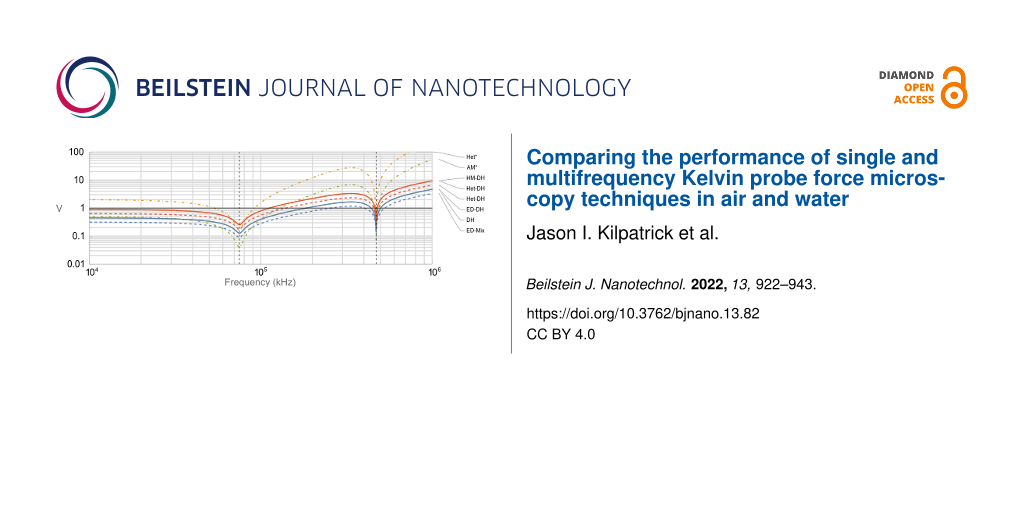
Since the transfer function of the cantilever is fundamental in determining the performance of a given KPFM mode at a given frequency, it is important to understand its influence. Figure 6 shows the frequency dependence of ![[Graphic 95]](/bjnano/content/inline/2190-4286-13-82-i166.svg?max-width=637&scale=1.18182) for air and water cases. Single-frequency modes are included for comparison. Note that previous calculations placed the drive frequencies such that the harmonics of the electrostatic response occurred in the desired locations with respect to the eigenmodes. For this figure, we calculate
for air and water cases. Single-frequency modes are included for comparison. Note that previous calculations placed the drive frequencies such that the harmonics of the electrostatic response occurred in the desired locations with respect to the eigenmodes. For this figure, we calculate ![[Graphic 96]](/bjnano/content/inline/2190-4286-13-82-i167.svg?max-width=637&scale=1.18182) such that the relevant electrostatic response occurs at the frequency stated on the x-axis. This means we divide the input frequency for Equation 17 and Equation 31 by two for comparison. We observe that the minimum bias occurs on the eigenmodes with ω1 having a smaller
such that the relevant electrostatic response occurs at the frequency stated on the x-axis. This means we divide the input frequency for Equation 17 and Equation 31 by two for comparison. We observe that the minimum bias occurs on the eigenmodes with ω1 having a smaller ![[Graphic 97]](/bjnano/content/inline/2190-4286-13-82-i168.svg?max-width=637&scale=1.18182) than ω2, as expected. The shape of the response for both air and water cases is proportional to N(ω)/G(ω). We also observe that there is a parallel relationship in
than ω2, as expected. The shape of the response for both air and water cases is proportional to N(ω)/G(ω). We also observe that there is a parallel relationship in ![[Graphic 98]](/bjnano/content/inline/2190-4286-13-82-i169.svg?max-width=637&scale=1.18182) between the multifrequency modes with fixed ratios. The ratio between purely electrical and mechanically coupled modes is Am/2z whilst the ratio between modes with the suffix DH and Mix is √2. Single-frequency modes exhibit a stronger frequency dependence with AM having the lowest
between the multifrequency modes with fixed ratios. The ratio between purely electrical and mechanically coupled modes is Am/2z whilst the ratio between modes with the suffix DH and Mix is √2. Single-frequency modes exhibit a stronger frequency dependence with AM having the lowest ![[Graphic 99]](/bjnano/content/inline/2190-4286-13-82-i170.svg?max-width=637&scale=1.18182) of any mode at the eigenmodes.
of any mode at the eigenmodes.
![[2190-4286-13-82-6]](/bjnano/content/figures/2190-4286-13-82-6.png?scale=2.0&max-width=1024&background=FFFFFF)
Figure 6:
Comparison of the minimum AC bias required for operation, ![[Graphic 100]](/bjnano/content/inline/2190-4286-13-82-i171.svg?max-width=637&scale=1.18182) as a function of frequency in (a) air and (b) water. Calculations are made for z = 10 nm. The vertical dashed black lines indicate eigenmode positions. *Designated single-frequency modes. VCPD = 0.1 V for single frequency modes. The solid black lines indicate
as a function of frequency in (a) air and (b) water. Calculations are made for z = 10 nm. The vertical dashed black lines indicate eigenmode positions. *Designated single-frequency modes. VCPD = 0.1 V for single frequency modes. The solid black lines indicate ![[Graphic 101]](/bjnano/content/inline/2190-4286-13-82-i172.svg?max-width=637&scale=1.18182) = 1.0 V. Lower values are better for all graphs.
= 1.0 V. Lower values are better for all graphs.
Figure 6:
Comparison of the minimum AC bias required for operation, as a function of frequency in (a) air an...
Conclusion
In this work, we have presented the derivation of equations that allow the performance of a range of single- and multifrequency KPFM modes to be directly compared quantitatively. The relative performance of each mode is then presented in air and water in order to allow us to identify a suitable candidate for performing KPFM-based experiments in liquid with optimal response whilst minimizing the required low VAC needed for operation in order to avoid the associated problems, for example, current flow, electrodeposition, or Faradaic reactions [9]. For this assessment, a number of simplifying assumptions have been made: (1) We use a simple spherical model of tip–sample capacitance [2,97] and do not consider the contributions from the rest of the cantilever. This would generally lead to an under-reporting of the superior voltage sensitivity (at the cost of lateral resolution) of the purely electrical modes in this work. (2) We consider both air and water as linear lossless dielectric media and do not consider additional properties such as electrodynamics or the effect of the tip–sample position relative to the position of the double layer. (3) We only compare frequency responses off resonance, ωoff, and for the first two eigenmodes of the cantilever and combinations thereof. The driving frequencies are chosen such that the first harmonic of the electrostatic response signal will occur either on ωoff (ωe ≪ ω1), or on ω1 or ω2. In practice, KPFM can be performed at any chosen frequency. (4) For modes including a mechanical excitation of the lever, the response is calculated at the mean tip–sample separation. The true instantaneous response would depend on the tip–sample separation during the oscillation cycle. (5) We consider the capacitive terms to be equivalent for different eigenmodes, allowing for a direct division of the electrostatic force harmonics in order to access CPD. Some authors have indicated that the capacitance contribution of the lever differs at higher eigenmodes due to the mode shape of the cantilever [17,60,63]. This would primarily affect the accuracy of CPD for purely electrical modes dependent on C′ as the mechanically coupled modes dependent on C″ have minimal cantilever contribution [101]. Any difference in capacitance (and therefore corrections that need to be applied) could be established by measuring the z dependence of the second harmonic of the electrostatic force for each eigenmode [29,83,98].
Whilst these simplifications are applied in this paper, the equations presented herein can be extended and applied to experiments with increased complexity. As such, we consider these equations to serve as the basis for planning KPFM-based experiments and assessing relative performance of KPFM-based modes. Furthermore, Table 3 in Appendix III provides a comprehensive guide to the various drive and detection schemes that are necessary to implement each of the KPFM modes presented in this paper along with a brief description of the advantages and disadvantages of each technique.
Clear trends are present in the comparison of the modes throughout: (1) Purely electrical modes require smaller VAC and have better CPD detection and SNR than their mechanically coupled analogues. Each of these performance metrics is decreased by a factor of Am/2z for the mechanically coupled analogues of the purely electrical modes. (2) DH modes suffer significantly from problems with frequency placement relative to the transfer function of the cantilever. This could be remedied by operation of these modes using a half-harmonic [40,82] approach, which would greatly improve performance and remove reliance of XGain at the expense of having to scan the sample twice (once for each harmonic of the electrostatic response) and the associated errors due to sample drift or other temporal changes in the state of the tip and/or the sample. (3) Performance is optimal when the first harmonic of the electrostatic force occurs on the first eigenmode. (4) Smaller VAC is required when operating in liquid environments due to the increased relative permittivity. We note that in the presence of ions there will be a strong z dependence, which may restrict practical operation to z ≤ R [107]. (5) Modes reliant upon Mix terms are superior in performance to those based on DH terms by a factor of √2.
As the transfer function of the cantilever significantly influences KPFM performance and multifrequency OL KPFM techniques become more popular for applications in liquid environments, the choice of cantilever geometry is becoming an increasingly important factor to consider in planning experiments and optimizing performance. Through mechanical design of the cantilever the placement of eigenmodes and their relative Qn/kn ratios can be optimized for increased performance of a given KPFM mode [108-110].
Whilst single-frequency KPFM modes are the most ubiquitous and easy to implement, their typical operation requires the application of a DC bias, which makes them unsuitable for applications in liquid environments. Even when these modes can be operated in an OL manner, they require explicit knowledge of C′ or C″, either through measurement or modeling, which can be difficult to establish in liquids in the presence of ions. Multifrequency OL KPFM-based approaches are therefore preferred in liquid environments. The ability to place multiple harmonics on eigenmodes to enhance performance in a single pass is preferable over multi-pass DH-based techniques. As such, ED and HM are the leading candidates for liquid operation. ED mixed modes with low bias requirements are a superior choice for larger (z > R) tip–sample separations whereas operation close to the surface is comparable to HM. For this case, the choice relies on the need for increased spatial resolution, which HM provides despite the dependency on C″. The use of Mix modes, where there is a contribution from both of the applied electrical drive signals, offers superior performance over DH-based modes of operation. As such, we conclude that ED-Mix and HM-Mix are the ideal candidates for KPFM-based measurements in liquid environments.
Appendix I: Calculation Parameters
For calculation parameters see Table 2.
Table 2: Parameters used for calculations (air and water).
| Constants | Value air (water) | Cantilever properties | Value air (water) |
| kB | 1.38064852 × 10⁻²³ J/K | f1 | 75,000 (30,000) Hz |
| e0 | 8.8541878 × 10⁻¹² F/m | ω1 | 2π f1 Hz |
| er | 1 (80) | ω2 | 4π2 f1 Hz |
| T | 300 K | Q1 | 200 (5) |
| Nd |
100 × 10−15 m/![[Graphic 102]](/bjnano/content/inline/2190-4286-13-82-i173.svg?max-width=637&scale=1.0)
|
Q2 | 600 (15) |
| B | 100 Hz | k1 | 2.8 N/m |
| VAC | 1.0 V | k2 | 110 N/m |
| VCPD | 0.1 V | Am | 5 nm |
| R | 10 nm | ||
Appendix II: Derivation of Performance Determining Equations
The noise of a cantilever under ambient conditions at frequency ω, in a given bandwidth B, is defined as
![[2190-4286-13-82-i1]](/bjnano/content/inline/2190-4286-13-82-i1.svg?max-width=590&scale=1.18182)
for the first two eigenmodes, where kB is Boltzmann's constant, T is the temperature, Nd is the detector noise, and ωn, kn, and Qn are, respectively, the resonance frequency, spring constant, and quality factor of the n-th eigenmode (n = 1, 2). The corresponding gain at a given frequency is then defined as
![[2190-4286-13-82-i2]](/bjnano/content/inline/2190-4286-13-82-i2.svg?max-width=590&scale=1.18182)
We note that more complex expressions for the transfer function of the cantilever are present in the literature and that these models may better represent the behavior of the lever in different environments [111-116].
A. Amplitude Modulation KPFM (AM)
In KPFM-based techniques, a bias is applied between a conductive AFM probe and a sample
![[2190-4286-13-82-i3]](/bjnano/content/inline/2190-4286-13-82-i3.svg?max-width=590&scale=1.18182)
where VDC is the DC bias and VAC is the AC bias applied at frequency ωe. Here, the bias may be applied either to the cantilever or to the sample. The application of ΔU results in an electrostatic force given by
![[2190-4286-13-82-i4]](/bjnano/content/inline/2190-4286-13-82-i4.svg?max-width=590&scale=1.18182)
where C′ is the capacitance gradient with respect to tip–sample distance, z, and ends on the tip–sample geometry (see section "Influence of Capacitance Gradient and Amplitude"). By combining Equation 3 and Equation 4 we can obtain force components at DC, ωe and 2ωe (assuming VDC = 0).
![[2190-4286-13-82-i5]](/bjnano/content/inline/2190-4286-13-82-i5.svg?max-width=590&scale=1.18182)
![[2190-4286-13-82-i6]](/bjnano/content/inline/2190-4286-13-82-i6.svg?max-width=590&scale=1.18182)
![[2190-4286-13-82-i7]](/bjnano/content/inline/2190-4286-13-82-i7.svg?max-width=590&scale=1.18182)
Thus, the amplitude responses at ωe and 2ωe are given as
![[2190-4286-13-82-i8]](/bjnano/content/inline/2190-4286-13-82-i8.svg?max-width=590&scale=1.18182)
![[2190-4286-13-82-i9]](/bjnano/content/inline/2190-4286-13-82-i9.svg?max-width=590&scale=1.18182)
In order to assess the performance of the various KPFM modes, we consider the conventional condition where the minimum detectable CPD, ![[Graphic 103]](/bjnano/content/inline/2190-4286-13-82-i174.svg?max-width=637&scale=1.18182) is defined as the condition under which SNR = 1 [2,53,56-59]. For AM-KPFM we can solve the general equation for a single-frequency response at ωe
is defined as the condition under which SNR = 1 [2,53,56-59]. For AM-KPFM we can solve the general equation for a single-frequency response at ωe
![[2190-4286-13-82-i10]](/bjnano/content/inline/2190-4286-13-82-i10.svg?max-width=590&scale=1.18182)
for VCPD. By substituting Equation 8 into Equation 10 we obtain
![[2190-4286-13-82-i11]](/bjnano/content/inline/2190-4286-13-82-i11.svg?max-width=590&scale=1.18182)
Similarly, we can rearrange Equation 11 for ![[Graphic 104]](/bjnano/content/inline/2190-4286-13-82-i175.svg?max-width=637&scale=1.18182) and obtain
and obtain
![[2190-4286-13-82-i12]](/bjnano/content/inline/2190-4286-13-82-i12.svg?max-width=590&scale=1.18182)
The SNR is then defined as
![[2190-4286-13-82-i13]](/bjnano/content/inline/2190-4286-13-82-i13.svg?max-width=590&scale=1.18182)
By substituting Equation 8 into Equation 13 we obtain
![[2190-4286-13-82-i14]](/bjnano/content/inline/2190-4286-13-82-i14.svg?max-width=590&scale=1.18182)
Here, the SNR is specific to OL operation as in CL the feedback loop will reduce ![[Graphic 105]](/bjnano/content/inline/2190-4286-13-82-i176.svg?max-width=637&scale=1.18182) through the application of a DC bias such that
through the application of a DC bias such that ![[Graphic 106]](/bjnano/content/inline/2190-4286-13-82-i177.svg?max-width=637&scale=1.18182) = N(ωe) (assuming ideal feedback and no instrument artefacts). Under these conditions, the SNR would always be 1 for CL operation.
= N(ωe) (assuming ideal feedback and no instrument artefacts). Under these conditions, the SNR would always be 1 for CL operation.
B. Dual Harmonic KPFM (DH)
In DH-KPFM the amplitude responses at ![[Graphic 107]](/bjnano/content/inline/2190-4286-13-82-i178.svg?max-width=637&scale=1.18182) and
and ![[Graphic 108]](/bjnano/content/inline/2190-4286-13-82-i179.svg?max-width=637&scale=1.18182) are measured and VCPD(DH) is determined as [80]
are measured and VCPD(DH) is determined as [80]
![[2190-4286-13-82-i15]](/bjnano/content/inline/2190-4286-13-82-i15.svg?max-width=590&scale=1.18182)
where s = ![[Graphic 170]](/bjnano/content/inline/2190-4286-13-82-i241.svg?max-width=637&scale=1.18182) (where
(where ![[Graphic 171]](/bjnano/content/inline/2190-4286-13-82-i242.svg?max-width=637&scale=1.18182) is the phase of the first harmonic electrical response) determines the sign of VCPD, and
is the phase of the first harmonic electrical response) determines the sign of VCPD, and
![[2190-4286-13-82-i16]](/bjnano/content/inline/2190-4286-13-82-i16.svg?max-width=590&scale=1.18182)
Whilst the ![[Graphic 109]](/bjnano/content/inline/2190-4286-13-82-i180.svg?max-width=637&scale=1.18182) for DH-KPFM is the same as Equation 11 for the first harmonic response, we are primarily interested in the performance of the techniques as a function of
for DH-KPFM is the same as Equation 11 for the first harmonic response, we are primarily interested in the performance of the techniques as a function of ![[Graphic 110]](/bjnano/content/inline/2190-4286-13-82-i181.svg?max-width=637&scale=1.18182) Here,
Here, ![[Graphic 111]](/bjnano/content/inline/2190-4286-13-82-i182.svg?max-width=637&scale=1.18182) is determined from the bias required to satisfy the SNR = 1 condition for
is determined from the bias required to satisfy the SNR = 1 condition for ![[Graphic 112]](/bjnano/content/inline/2190-4286-13-82-i183.svg?max-width=637&scale=1.18182) whereby
whereby
![[2190-4286-13-82-i17]](/bjnano/content/inline/2190-4286-13-82-i17.svg?max-width=590&scale=1.18182)
Substituting Equation 17 into Equation 11 we obtain ![[Graphic 113]](/bjnano/content/inline/2190-4286-13-82-i184.svg?max-width=637&scale=1.18182) under conditions where
under conditions where ![[Graphic 114]](/bjnano/content/inline/2190-4286-13-82-i185.svg?max-width=637&scale=1.18182) and
and
![[2190-4286-13-82-i18]](/bjnano/content/inline/2190-4286-13-82-i18.svg?max-width=590&scale=1.18182)
SNR is then obtained from the root sum squared of ![[Graphic 115]](/bjnano/content/inline/2190-4286-13-82-i186.svg?max-width=637&scale=1.418184) and
and ![[Graphic 116]](/bjnano/content/inline/2190-4286-13-82-i187.svg?max-width=637&scale=1.418184) resulting in
resulting in
![[2190-4286-13-82-i19]](/bjnano/content/inline/2190-4286-13-82-i19.svg?max-width=590&scale=1.18182)
C. Heterodyne-KPFM (Het)
For heterodyne-KPFM, both mechanical, ωm, and electrical, ωe, signals are applied. Under conditions where VDC = 0 (typical of OL operation) we obtain
![[2190-4286-13-82-i20]](/bjnano/content/inline/2190-4286-13-82-i20.svg?max-width=590&scale=1.18182)
![[2190-4286-13-82-i21]](/bjnano/content/inline/2190-4286-13-82-i21.svg?max-width=590&scale=1.18182)
![[2190-4286-13-82-i22]](/bjnano/content/inline/2190-4286-13-82-i22.svg?max-width=590&scale=1.18182)
![[2190-4286-13-82-i23]](/bjnano/content/inline/2190-4286-13-82-i23.svg?max-width=590&scale=1.18182)
where C″ is the derivative of the capacitance gradient with respect to z. Thus, the amplitudes are given by
![[2190-4286-13-82-i24]](/bjnano/content/inline/2190-4286-13-82-i24.svg?max-width=590&scale=1.18182)
![[2190-4286-13-82-i25]](/bjnano/content/inline/2190-4286-13-82-i25.svg?max-width=590&scale=1.18182)
![[2190-4286-13-82-i26]](/bjnano/content/inline/2190-4286-13-82-i26.svg?max-width=590&scale=1.18182)
![[2190-4286-13-82-i27]](/bjnano/content/inline/2190-4286-13-82-i27.svg?max-width=590&scale=1.18182)
Generally, Het-KPFM is operated in CL employing a feedback loop applying a DC bias to the system to nullify the response at ![[Graphic 117]](/bjnano/content/inline/2190-4286-13-82-i188.svg?max-width=637&scale=1.18182) Alternatively, knowledge of the capacitance gradient and transfer function of the cantilever would allow the CPD to be determined without employing a feedback loop. For Het-KPFM where only
Alternatively, knowledge of the capacitance gradient and transfer function of the cantilever would allow the CPD to be determined without employing a feedback loop. For Het-KPFM where only ![[Graphic 118]](/bjnano/content/inline/2190-4286-13-82-i189.svg?max-width=637&scale=1.18182) is measured
is measured
![[2190-4286-13-82-i28]](/bjnano/content/inline/2190-4286-13-82-i28.svg?max-width=590&scale=1.18182)
where
![[2190-4286-13-82-i29]](/bjnano/content/inline/2190-4286-13-82-i29.svg?max-width=590&scale=1.18182)
VCPD can also be obtained for OL operation of Het-KPFM by dividing Equation 26 by Equation 27 (analogous to DH-KPFM) to obtain
![[2190-4286-13-82-i30]](/bjnano/content/inline/2190-4286-13-82-i30.svg?max-width=590&scale=1.18182)
where
![[2190-4286-13-82-i31]](/bjnano/content/inline/2190-4286-13-82-i31.svg?max-width=590&scale=1.18182)
Thus, measuring signals at ωm ± ωe and ωm ± 2ωe is required. Substituting Equation 31 into Equation 28 we obtain
![[2190-4286-13-82-i32]](/bjnano/content/inline/2190-4286-13-82-i32.svg?max-width=590&scale=1.18182)
The SNR is then obtained from the root sum squared of ![[Graphic 119]](/bjnano/content/inline/2190-4286-13-82-i190.svg?max-width=637&scale=1.18182) and
and ![[Graphic 120]](/bjnano/content/inline/2190-4286-13-82-i191.svg?max-width=637&scale=1.18182) resulting in
resulting in
![[2190-4286-13-82-i33]](/bjnano/content/inline/2190-4286-13-82-i33.svg?max-width=590&scale=1.18182)
D. Electrodyne-KPFM (ED)
For electrodyne-KPFM, two electrical signals, ωe1 and ωe2, are applied and these generate an array of mixing products. Here,
![[2190-4286-13-82-i34]](/bjnano/content/inline/2190-4286-13-82-i34.svg?max-width=590&scale=1.18182)
Substituting Equation 34 into Equation 4 we obtain [51,83]
![[2190-4286-13-82-i35]](/bjnano/content/inline/2190-4286-13-82-i35.svg?max-width=590&scale=1.18182)
![[2190-4286-13-82-i36]](/bjnano/content/inline/2190-4286-13-82-i36.svg?max-width=590&scale=1.18182)
![[2190-4286-13-82-i37]](/bjnano/content/inline/2190-4286-13-82-i37.svg?max-width=590&scale=1.18182)
![[2190-4286-13-82-i38]](/bjnano/content/inline/2190-4286-13-82-i38.svg?max-width=590&scale=1.18182)
where ωe1 > ωe2. The amplitude responses are thus
![[2190-4286-13-82-i39]](/bjnano/content/inline/2190-4286-13-82-i39.svg?max-width=590&scale=1.18182)
![[2190-4286-13-82-i40]](/bjnano/content/inline/2190-4286-13-82-i40.svg?max-width=590&scale=1.18182)
![[2190-4286-13-82-i41]](/bjnano/content/inline/2190-4286-13-82-i41.svg?max-width=590&scale=1.18182)
where ωmix = ωe1 ± ωe2. Here, we will assume VAC = VAC1 = VAC2. Thus, VCPD(ED-DH) can be obtained by combinations of ![[Graphic 121]](/bjnano/content/inline/2190-4286-13-82-i192.svg?max-width=637&scale=1.18182) and
and ![[Graphic 122]](/bjnano/content/inline/2190-4286-13-82-i193.svg?max-width=637&scale=1.18182) in a similar manner to DH-KPFM [51] where
in a similar manner to DH-KPFM [51] where
![[2190-4286-13-82-i42]](/bjnano/content/inline/2190-4286-13-82-i42.svg?max-width=590&scale=1.18182)
or by combining ![[Graphic 123]](/bjnano/content/inline/2190-4286-13-82-i194.svg?max-width=637&scale=1.18182) with
with ![[Graphic 124]](/bjnano/content/inline/2190-4286-13-82-i195.svg?max-width=637&scale=1.18182) such that
such that
![[2190-4286-13-82-i43]](/bjnano/content/inline/2190-4286-13-82-i43.svg?max-width=590&scale=1.18182)
We can then determine the ![[Graphic 125]](/bjnano/content/inline/2190-4286-13-82-i196.svg?max-width=637&scale=1.18182) for
for ![[Graphic 126]](/bjnano/content/inline/2190-4286-13-82-i197.svg?max-width=637&scale=1.18182) such that
such that
![[2190-4286-13-82-i44]](/bjnano/content/inline/2190-4286-13-82-i44.svg?max-width=590&scale=1.18182)
and thus
![[2190-4286-13-82-i45]](/bjnano/content/inline/2190-4286-13-82-i45.svg?max-width=590&scale=1.18182)
Similarly, for the case of ![[Graphic 127]](/bjnano/content/inline/2190-4286-13-82-i198.svg?max-width=637&scale=1.18182) we can obtain
we can obtain
![[2190-4286-13-82-i46]](/bjnano/content/inline/2190-4286-13-82-i46.svg?max-width=590&scale=1.18182)
which results in
![[2190-4286-13-82-i47]](/bjnano/content/inline/2190-4286-13-82-i47.svg?max-width=590&scale=1.18182)
and the resulting SNR is then obtained from the root sum squared of ![[Graphic 128]](/bjnano/content/inline/2190-4286-13-82-i199.svg?max-width=637&scale=1.18182) and
and ![[Graphic 129]](/bjnano/content/inline/2190-4286-13-82-i200.svg?max-width=637&scale=1.18182) resulting in
resulting in
![[2190-4286-13-82-i48]](/bjnano/content/inline/2190-4286-13-82-i48.svg?max-width=590&scale=1.18182)
Similarly, using the root sum squared of ![[Graphic 130]](/bjnano/content/inline/2190-4286-13-82-i201.svg?max-width=637&scale=1.18182) and
and ![[Graphic 131]](/bjnano/content/inline/2190-4286-13-82-i202.svg?max-width=637&scale=1.18182) we obtain
we obtain
![[2190-4286-13-82-i49]](/bjnano/content/inline/2190-4286-13-82-i49.svg?max-width=590&scale=1.18182)
E. Harmonic Mixing-KPFM (HM)
When Equation 34 is combined with ωm, the resulting frequency components of the electrostatic force become [10,51,83]
![[2190-4286-13-82-i50]](/bjnano/content/inline/2190-4286-13-82-i50.svg?max-width=590&scale=1.18182)
![[2190-4286-13-82-i51]](/bjnano/content/inline/2190-4286-13-82-i51.svg?max-width=590&scale=1.18182)
![[2190-4286-13-82-i52]](/bjnano/content/inline/2190-4286-13-82-i52.svg?max-width=590&scale=1.18182)
![[2190-4286-13-82-i53]](/bjnano/content/inline/2190-4286-13-82-i53.svg?max-width=590&scale=1.18182)
![[2190-4286-13-82-i54]](/bjnano/content/inline/2190-4286-13-82-i54.svg?max-width=590&scale=1.18182)
![[2190-4286-13-82-i55]](/bjnano/content/inline/2190-4286-13-82-i55.svg?max-width=590&scale=1.18182)
![[2190-4286-13-82-i56]](/bjnano/content/inline/2190-4286-13-82-i56.svg?max-width=590&scale=1.18182)
![[2190-4286-13-82-i57]](/bjnano/content/inline/2190-4286-13-82-i57.svg?max-width=590&scale=1.18182)
where ωe1 > ωe2. The amplitude responses are thus
![[2190-4286-13-82-i58]](/bjnano/content/inline/2190-4286-13-82-i58.svg?max-width=590&scale=1.18182)
![[2190-4286-13-82-i59]](/bjnano/content/inline/2190-4286-13-82-i59.svg?max-width=590&scale=1.18182)
![[2190-4286-13-82-i60]](/bjnano/content/inline/2190-4286-13-82-i60.svg?max-width=590&scale=1.18182)
![[2190-4286-13-82-i61]](/bjnano/content/inline/2190-4286-13-82-i61.svg?max-width=590&scale=1.18182)
![[2190-4286-13-82-i62]](/bjnano/content/inline/2190-4286-13-82-i62.svg?max-width=590&scale=1.18182)
![[2190-4286-13-82-i63]](/bjnano/content/inline/2190-4286-13-82-i63.svg?max-width=590&scale=1.18182)
where ωmix = ωe1 ± ωe2. Again, we will assume VAC = VAC1 = VAC2. Thus, VCPD may be obtained using the same approach as Equation 41 and Equation 42 using signals that are not modulated by ωm.
We can also obtain VCPD using ![[Graphic 132]](/bjnano/content/inline/2190-4286-13-82-i203.svg?max-width=637&scale=1.18182) and
and ![[Graphic 133]](/bjnano/content/inline/2190-4286-13-82-i204.svg?max-width=637&scale=1.18182) which have a dependence on C″, to yield [51]
which have a dependence on C″, to yield [51]
![[2190-4286-13-82-i64]](/bjnano/content/inline/2190-4286-13-82-i64.svg?max-width=590&scale=1.18182)
or by using ![[Graphic 134]](/bjnano/content/inline/2190-4286-13-82-i205.svg?max-width=637&scale=1.18182) and
and ![[Graphic 135]](/bjnano/content/inline/2190-4286-13-82-i206.svg?max-width=637&scale=1.18182) we can obtain
we can obtain
![[2190-4286-13-82-i65]](/bjnano/content/inline/2190-4286-13-82-i65.svg?max-width=590&scale=1.18182)
We can determine the ![[Graphic 136]](/bjnano/content/inline/2190-4286-13-82-i207.svg?max-width=637&scale=1.18182) for
for ![[Graphic 137]](/bjnano/content/inline/2190-4286-13-82-i208.svg?max-width=637&scale=1.18182) such that
such that
![[2190-4286-13-82-i66]](/bjnano/content/inline/2190-4286-13-82-i66.svg?max-width=590&scale=1.18182)
and thus
![[2190-4286-13-82-i67]](/bjnano/content/inline/2190-4286-13-82-i67.svg?max-width=590&scale=1.18182)
We can determine the ![[Graphic 138]](/bjnano/content/inline/2190-4286-13-82-i209.svg?max-width=637&scale=1.18182) for
for ![[Graphic 139]](/bjnano/content/inline/2190-4286-13-82-i210.svg?max-width=637&scale=1.18182) such that
such that
![[2190-4286-13-82-i68]](/bjnano/content/inline/2190-4286-13-82-i68.svg?max-width=590&scale=1.18182)
and thus
![[2190-4286-13-82-i69]](/bjnano/content/inline/2190-4286-13-82-i69.svg?max-width=590&scale=1.18182)
Here, we note that
![[Graphic 140]](/bjnano/content/inline/2190-4286-13-82-i211.svg?max-width=637&scale=1.18182)
The resulting SNR is then obtained from the root sum squared of
![[Graphic 141]](/bjnano/content/inline/2190-4286-13-82-i212.svg?max-width=637&scale=1.3000021)
and
![[Graphic 142]](/bjnano/content/inline/2190-4286-13-82-i213.svg?max-width=637&scale=1.3000021)
resulting in
![[2190-4286-13-82-i70]](/bjnano/content/inline/2190-4286-13-82-i70.svg?max-width=590&scale=1.18182)
Similarly, when using the root sum squared of
![[Graphic 143]](/bjnano/content/inline/2190-4286-13-82-i214.svg?max-width=637&scale=1.18182)
and
![[Graphic 144]](/bjnano/content/inline/2190-4286-13-82-i215.svg?max-width=637&scale=1.18182)
we obtain
![[2190-4286-13-82-i71]](/bjnano/content/inline/2190-4286-13-82-i71.svg?max-width=590&scale=1.18182)
Appendix III: Summary of Drive and Detection Schemes
For a summary of drive and detection schemes see Table 3.
Table 3: Summary of drive and detection (Det.) schemes.a
| Mode |
![[Graphic 145]](/bjnano/content/inline/2190-4286-13-82-i216.svg?max-width=637&scale=1.0)
|
![[Graphic 146]](/bjnano/content/inline/2190-4286-13-82-i217.svg?max-width=637&scale=1.0)
|
![[Graphic 147]](/bjnano/content/inline/2190-4286-13-82-i218.svg?max-width=637&scale=1.0)
Drive |
![[Graphic 148]](/bjnano/content/inline/2190-4286-13-82-i219.svg?max-width=637&scale=1.0)
Det. |
VCPD ∝ | C′/C″ | VAC ∝ | Advantages | Disadvantages |
| AMb | ω1 | ω2c | ω1 | ω1 |
![[Graphic 149]](/bjnano/content/inline/2190-4286-13-82-i220.svg?max-width=637&scale=1.0)
|
C′ | Q1/k1 |
widely available
high sensitivity |
low spatial resolution |
| ω2 | ω1c | ω2 | ω2 |
![[Graphic 150]](/bjnano/content/inline/2190-4286-13-82-i221.svg?max-width=637&scale=1.0)
|
C′ | Q2/k2 | |||
| DH | ω1 | ω2c | ω1 |
ω1
2ω1 |
![[Graphic 151]](/bjnano/content/inline/2190-4286-13-82-i222.svg?max-width=637&scale=1.0)
|
C′ | Q1/k1 | single pass scan compatible |
low spatial resolution
frequency placement poor SNR reliance on XGain |
| ω2 | ω1c | ω2 |
ω2
2ω2 |
![[Graphic 152]](/bjnano/content/inline/2190-4286-13-82-i223.svg?max-width=637&scale=1.0)
|
C′ | Q2/k2 | |||
| ED-DH | ω1 | – |
ω1
ω2/2 |
ω1
ω2 |
![[Graphic 153]](/bjnano/content/inline/2190-4286-13-82-i224.svg?max-width=637&scale=1.0)
|
C′ | Q1/k1 |
flexible frequency placement
high bandwidth |
low spatial resolution
difficult to use in single pass reliance on XGain |
| ω2 | – |
ω2
ω1/2 |
ω2
ω1 |
![[Graphic 154]](/bjnano/content/inline/2190-4286-13-82-i225.svg?max-width=637&scale=1.0)
|
C′ | Q2/k2 | |||
| ED-Mix | ω1 | – |
ω1
(ω2 ± ω1) |
ω1
ω2 |
![[Graphic 155]](/bjnano/content/inline/2190-4286-13-82-i226.svg?max-width=637&scale=1.0)
|
C′ | Q1/k1 |
sensitivity > ED-DH
flexible frequency placement high bandwidth |
low spatial resolution
difficult to use in single pass reliance on XGain |
| ω2 | – |
ω2
(ω2 ± ω1) |
ω2
ω1 |
![[Graphic 156]](/bjnano/content/inline/2190-4286-13-82-i227.svg?max-width=637&scale=1.0)
|
C′ | Q2/k2 | |||
| Hetb | ω1 | ω2 | (ω2 ± ω1) | ω1 |
![[Graphic 157]](/bjnano/content/inline/2190-4286-13-82-i228.svg?max-width=637&scale=1.0)
|
C″ | AmQ1/k1 |
sensitivity > FM-KPFM
high bandwidth high spatial resolution |
sensitivity < AM
higher bias required |
| ω2 | ω1 | (ω2 ± ω1) | ω2 |
![[Graphic 158]](/bjnano/content/inline/2190-4286-13-82-i229.svg?max-width=637&scale=1.0)
|
C″ | AmQ2/k2 | |||
| Het-DH | ω1 | ω2 | (ω2 ± ω1) |
ω1
2ω1 |
![[Graphic 159]](/bjnano/content/inline/2190-4286-13-82-i230.svg?max-width=637&scale=1.0)
|
C″ | AmQ1/k1 |
high bandwidth
high spatial resolution |
sensitivity < DH
frequency placement reliance on XGain |
| ω2 | ω1 | (ω2 ± ω1) |
ω2
1ω2 |
![[Graphic 160]](/bjnano/content/inline/2190-4286-13-82-i231.svg?max-width=637&scale=1.0)
|
C″ | AmQ2/k2 | |||
| HM-DH | ω1 | ωn |
(ωn ± ω1)
(ωn ± ω2/2) |
ω1
ω2 |
![[Graphic 161]](/bjnano/content/inline/2190-4286-13-82-i232.svg?max-width=637&scale=1.0)
|
C″ | AmQ1/k1 |
flexible frequency placement
high bandwidth high spatial resolution |
sensitivity < ED-DH
frequency placement reliance on XGain |
| ω2 | ωn |
(ωn ± ω2)
(ωn ± ω1/2) |
ω2
ω1 |
![[Graphic 162]](/bjnano/content/inline/2190-4286-13-82-i233.svg?max-width=637&scale=1.0)
|
C″ | AmQ2/k2 | |||
| HM-Mix | ω1 | ωn |
(ωn ± ω1)
(ωn ± ω2) |
ω1
ω2 |
![[Graphic 163]](/bjnano/content/inline/2190-4286-13-82-i234.svg?max-width=637&scale=1.0)
|
C″ | AmQ1/k1 |
flexible frequency placement
high bandwidth high spatial resolution |
sensitivity < ED-Mix
reliance on XGain |
| ω2 | ωn |
(ωn ± ω2)
(ωn ± ω1) |
ω2
ω1 |
![[Graphic 164]](/bjnano/content/inline/2190-4286-13-82-i235.svg?max-width=637&scale=1.0)
|
C″ | AmQ2/k2 | |||
aωn = mechanical oscillation, on another eigenmode or off resonance, at a frequency which does not interfere with electrical drive or detection and results in an oscillation amplitude, Am. Off-resonance conditions imply all electrical detection frequencies ω → 0 Hz. bTechniques that would typically be operated in a closed loop configuration. cThe drive is optional.
References
-
Binnig, G.; Quate, C. F.; Gerber, C. Phys. Rev. Lett. 1986, 56, 930–933. doi:10.1103/physrevlett.56.930
Return to citation in text: [1] -
Nonnenmacher, M.; O’Boyle, M. P.; Wickramasinghe, H. K. Appl. Phys. Lett. 1991, 58, 2921–2923. doi:10.1063/1.105227
Return to citation in text: [1] [2] [3] [4] [5] [6] [7] -
Shen, C., Ed. Atomic Force Microscopy for Energy Research, 1st ed.; CRC Press: Boca Raton, FL, USA, 2022. doi:10.1201/9781003174042
Return to citation in text: [1] -
Lee, H.; Lee, W.; Lee, J. H.; Yoon, D. S. J. Nanomater. 2016, 4209130. doi:10.1155/2016/4209130
Return to citation in text: [1] -
Moores, B.; Hane, F.; Eng, L.; Leonenko, Z. Ultramicroscopy 2010, 110, 708–711. doi:10.1016/j.ultramic.2010.02.036
Return to citation in text: [1] -
Melitz, W.; Shen, J.; Kummel, A. C.; Lee, S. Surf. Sci. Rep. 2011, 66, 1–27. doi:10.1016/j.surfrep.2010.10.001
Return to citation in text: [1] [2] -
Barth, C.; Foster, A. S.; Henry, C. R.; Shluger, A. L. Adv. Mater. (Weinheim, Ger.) 2011, 23, 477–501. doi:10.1002/adma.201002270
Return to citation in text: [1] -
Cheong, L.-Z.; Zhao, W.; Song, S.; Shen, C. Acta Biomater. 2019, 99, 33–52. doi:10.1016/j.actbio.2019.08.023
Return to citation in text: [1] -
Collins, L.; Kilpatrick, J. I.; Kalinin, S. V.; Rodriguez, B. J. Rep. Prog. Phys. 2018, 81, 086101. doi:10.1088/1361-6633/aab560
Return to citation in text: [1] [2] [3] [4] -
Axt, A.; Hermes, I. M.; Bergmann, V. W.; Tausendpfund, N.; Weber, S. A. L. Beilstein J. Nanotechnol. 2018, 9, 1809–1819. doi:10.3762/bjnano.9.172
Return to citation in text: [1] [2] [3] [4] [5] [6] [7] [8] [9] [10] [11] [12] -
Coffey, D. C.; Ginger, D. S. Nat. Mater. 2006, 5, 735–740. doi:10.1038/nmat1712
Return to citation in text: [1] [2] [3] -
Giridharagopal, R.; Rayermann, G. E.; Shao, G.; Moore, D. T.; Reid, O. G.; Tillack, A. F.; Masiello, D. J.; Ginger, D. S. Nano Lett. 2012, 12, 893–898. doi:10.1021/nl203956q
Return to citation in text: [1] [2] [3] -
Murawski, J.; Graupner, T.; Milde, P.; Raupach, R.; Zerweck-Trogisch, U.; Eng, L. M. J. Appl. Phys. 2015, 118, 154302. doi:10.1063/1.4933289
Return to citation in text: [1] [2] [3] [4] -
Collins, L.; Ahmadi, M.; Wu, T.; Hu, B.; Kalinin, S. V.; Jesse, S. ACS Nano 2017, 11, 8717–8729. doi:10.1021/acsnano.7b02114
Return to citation in text: [1] [2] [3] [4] [5] -
Zerweck, U.; Loppacher, C.; Otto, T.; Grafström, S.; Eng, L. M. Phys. Rev. B 2005, 71, 125424. doi:10.1103/physrevb.71.125424
Return to citation in text: [1] -
Colchero, J.; Gil, A.; Baró, A. M. Phys. Rev. B 2001, 64, 245403. doi:10.1103/physrevb.64.245403
Return to citation in text: [1] [2] -
Ding, X. D.; An, J.; Xu, J. B.; Li, C.; Zeng, R. Y. Appl. Phys. Lett. 2009, 94, 223109. doi:10.1063/1.3147198
Return to citation in text: [1] [2] [3] [4] -
Cadena, M. J.; Reifenberger, R. G.; Raman, A. Nanotechnology 2018, 29, 405702. doi:10.1088/1361-6528/aacfdc
Return to citation in text: [1] -
Jakob, D. S.; Wang, H.; Xu, X. G. ACS Nano 2020, 14, 4839–4848. doi:10.1021/acsnano.0c00767
Return to citation in text: [1] [2] [3] -
Aubriet, V.; Courouble, K.; Bardagot, O.; Demadrille, R.; Borowik, Ł.; Grévin, B. Nanotechnology 2022, 33, 225401. doi:10.1088/1361-6528/ac5542
Return to citation in text: [1] [2] -
Miyahara, Y.; Roy-Gobeil, A.; Grutter, P. Nanotechnology 2017, 28, 064001. doi:10.1088/1361-6528/aa5261
Return to citation in text: [1] -
Behn, W. A.; Krebs, Z. J.; Smith, K. J.; Watanabe, K.; Taniguchi, T.; Brar, V. W. Nano Lett. 2021, 21, 5013–5020. doi:10.1021/acs.nanolett.1c00791
Return to citation in text: [1] [2] -
Gross, L.; Schuler, B.; Pavliček, N.; Fatayer, S.; Majzik, Z.; Moll, N.; Peña, D.; Meyer, G. Angew. Chem., Int. Ed. 2018, 57, 3888–3908. doi:10.1002/anie.201703509
Return to citation in text: [1] -
Gross, L.; Schuler, B.; Mohn, F.; Moll, N.; Pavliček, N.; Steurer, W.; Scivetti, I.; Kotsis, K.; Persson, M.; Meyer, G. Phys. Rev. B 2014, 90, 155455. doi:10.1103/physrevb.90.155455
Return to citation in text: [1] -
Zhong, Q.; Li, X.; Zhang, H.; Chi, L. Surf. Sci. Rep. 2020, 75, 100509. doi:10.1016/j.surfrep.2020.100509
Return to citation in text: [1] -
Wagner, C.; Green, M. F. B.; Maiworm, M.; Leinen, P.; Esat, T.; Ferri, N.; Friedrich, N.; Findeisen, R.; Tkatchenko, A.; Temirov, R.; Tautz, F. S. Nat. Mater. 2019, 18, 853–859. doi:10.1038/s41563-019-0382-8
Return to citation in text: [1] -
Schuler, B.; Liu, S.-X.; Geng, Y.; Decurtins, S.; Meyer, G.; Gross, L. Nano Lett. 2014, 14, 3342–3346. doi:10.1021/nl500805x
Return to citation in text: [1] -
Collins, L.; Kilpatrick, J. I.; Weber, S. A. L.; Tselev, A.; Vlassiouk, I. V.; Ivanov, I. N.; Jesse, S.; Kalinin, S. V.; Rodriguez, B. J. Nanotechnology 2013, 24, 475702. doi:10.1088/0957-4484/24/47/475702
Return to citation in text: [1] [2] [3] -
Kilpatrick, J. I.; Collins, L.; Weber, S. A. L.; Rodriguez, B. J. Rev. Sci. Instrum. 2018, 89, 123708. doi:10.1063/1.5025432
Return to citation in text: [1] [2] [3] [4] [5] [6] -
Takeuchi, O.; Ohrai, Y.; Yoshida, S.; Shigekawa, H. Jpn. J. Appl. Phys., Part 1 2007, 46, 5626–5630. doi:10.1143/jjap.46.5626
Return to citation in text: [1] [2] -
Yoshida, S.; Kikuchi, J.; Kanitani, Y.; Takeuchi, O.; Oigawa, H.; Shigekawa, H. e-J. Surf. Sci. Nanotechnol. 2006, 4, 192–196. doi:10.1380/ejssnt.2006.192
Return to citation in text: [1] -
Sommerhalter, C.; Glatzel, T.; Matthes, T. W.; Jäger-Waldau, A.; Lux-Steiner, M. C. Appl. Surf. Sci. 2000, 157, 263–268. doi:10.1016/s0169-4332(99)00537-1
Return to citation in text: [1] -
Kobayashi, N.; Asakawa, H.; Fukuma, T. J. Appl. Phys. 2011, 110, 044315. doi:10.1063/1.3625230
Return to citation in text: [1] -
Kobayashi, N.; Asakawa, H.; Fukuma, T. Rev. Sci. Instrum. 2012, 83, 033709. doi:10.1063/1.3698207
Return to citation in text: [1] -
Hirata, K.; Kitagawa, T.; Miyazawa, K.; Okamoto, T.; Fukunaga, A.; Takatoh, C.; Fukuma, T. Nanoscale 2018, 10, 14736–14746. doi:10.1039/c8nr03600d
Return to citation in text: [1] -
Butt, H.-J.; Jaschke, M. Nanotechnology 1995, 6, 1–7. doi:10.1088/0957-4484/6/1/001
Return to citation in text: [1] [2] [3] -
Putman, C. A. J.; De Grooth, B. G.; Van Hulst, N. F.; Greve, J. J. Appl. Phys. 1992, 72, 6–12. doi:10.1063/1.352149
Return to citation in text: [1] -
Barbet, S.; Popoff, M.; Diesinger, H.; Deresmes, D.; Théron, D.; Mélin, T. J. Appl. Phys. 2014, 115, 144313. doi:10.1063/1.4870710
Return to citation in text: [1] -
Mélin, T.; Barbet, S.; Diesinger, H.; Théron, D.; Deresmes, D. Rev. Sci. Instrum. 2011, 82, 036101. doi:10.1063/1.3516046
Return to citation in text: [1] -
Guo, S.; Kalinin, S. V.; Jesse, S. Nanotechnology 2012, 23, 125704. doi:10.1088/0957-4484/23/12/125704
Return to citation in text: [1] [2] [3] [4] -
Borgani, R.; Pallon, L. K. H.; Hedenqvist, M. S.; Gedde, U. W.; Haviland, D. B. Nano Lett. 2016, 16, 5934–5937. doi:10.1021/acs.nanolett.6b02920
Return to citation in text: [1] -
Borgani, R. Probing Nonlinear Electrical Properties at the Nanoscale : Studies in Multifrequency AFM. Ph.D. Thesis, KTH Royal Institute of Technology, Stockholm, Sweden, 2018.
Return to citation in text: [1] [2] [3] [4] [5] -
Grévin, B.; Bardagot, O.; Demadrille, R. Beilstein J. Nanotechnol. 2020, 11, 323–337. doi:10.3762/bjnano.11.24
Return to citation in text: [1] -
Reid, O. G.; Rayermann, G. E.; Coffey, D. C.; Ginger, D. S. J. Phys. Chem. C 2010, 114, 20672–20677. doi:10.1021/jp1056607
Return to citation in text: [1] -
Murawski, J. Time-Resolved Kelvin Probe Force Microscopy of Nanostructured Devices. Ph.D. Thesis, Institut für Angewandte Physik der Technischen Universität Dresden, Dresden, Germany, 2016.
Return to citation in text: [1] -
Mascaro, A.; Miyahara, Y.; Enright, T.; Dagdeviren, O. E.; Grütter, P. Beilstein J. Nanotechnol. 2019, 10, 617–633. doi:10.3762/bjnano.10.62
Return to citation in text: [1] -
Sadewasser, S.; Nicoara, N. Time-Resolved Electrostatic and Kelvin Probe Force Microscopy. In Kelvin Probe Force Microscopy: From Single Charge Detection to Device Characterization; Sadewasser, S.; Glatzel, T., Eds.; Springer International Publishing: Cham, Switzerland, 2018; pp 119–143. doi:10.1007/978-3-319-75687-5
Return to citation in text: [1] -
Collins, L.; Belianinov, A.; Somnath, S.; Rodriguez, B. J.; Balke, N.; Kalinin, S. V.; Jesse, S. Nanotechnology 2016, 27, 105706. doi:10.1088/0957-4484/27/10/105706
Return to citation in text: [1] [2] [3] -
Collins, L.; Belianinov, A.; Somnath, S.; Balke, N.; Kalinin, S. V.; Jesse, S. Sci. Rep. 2016, 6, 30557. doi:10.1038/srep30557
Return to citation in text: [1] [2] [3] -
Collins, L.; Ahmadi, M.; Qin, J.; Liu, Y.; Ovchinnikova, O. S.; Hu, B.; Jesse, S.; Kalinin, S. V. Nanotechnology 2018, 29, 445703. doi:10.1088/1361-6528/aad873
Return to citation in text: [1] [2] [3] -
Borgani, R.; Forchheimer, D.; Bergqvist, J.; Thorén, P.-A.; Inganäs, O.; Haviland, D. B. Appl. Phys. Lett. 2014, 105, 143113. doi:10.1063/1.4897966
Return to citation in text: [1] [2] [3] [4] [5] [6] -
Stan, G.; Namboodiri, P. Beilstein J. Nanotechnol. 2021, 12, 1115–1126. doi:10.3762/bjnano.12.83
Return to citation in text: [1] [2] [3] -
Ma, Z.-M.; Mu, J.-L.; Tang, J.; Xue, H.; Zhang, H.; Xue, C.-Y.; Liu, J.; Li, Y.-J. Nanoscale Res. Lett. 2013, 8, 532. doi:10.1186/1556-276x-8-532
Return to citation in text: [1] [2] [3] [4] [5] [6] [7] -
Smith, D. P. E. Rev. Sci. Instrum. 1995, 66, 3191–3195. doi:10.1063/1.1145550
Return to citation in text: [1] -
Walters, D. A.; Cleveland, J. P.; Thomson, N. H.; Hansma, P. K.; Wendman, M. A.; Gurley, G.; Elings, V. Rev. Sci. Instrum. 1996, 67, 3583–3590. doi:10.1063/1.1147177
Return to citation in text: [1] -
Li, G.; Mao, B.; Lan, F.; Liu, L. Rev. Sci. Instrum. 2012, 83, 113701. doi:10.1063/1.4761922
Return to citation in text: [1] [2] [3] [4] -
Sugawara, Y.; Kou, L.; Ma, Z.; Kamijo, T.; Naitoh, Y.; Jun Li, Y. Appl. Phys. Lett. 2012, 100, 223104. doi:10.1063/1.4723697
Return to citation in text: [1] [2] [3] [4] [5] [6] [7] [8] -
Garrett, J. L.; Munday, J. N. Nanotechnology 2016, 27, 245705. doi:10.1088/0957-4484/27/24/245705
Return to citation in text: [1] [2] [3] [4] [5] [6] [7] [8] [9] [10] [11] [12] -
Giessibl, F. J. Rev. Mod. Phys. 2003, 75, 949–983. doi:10.1103/revmodphys.75.949
Return to citation in text: [1] [2] [3] -
Lai, J.; Wang, C.; Xing, Z.; Lu, S.; Chen, Q.; Chen, L. Ultramicroscopy 2021, 230, 113399. doi:10.1016/j.ultramic.2021.113399
Return to citation in text: [1] [2] [3] [4] [5] -
Ding, X. D.; Li, C.; Liang, Z. W.; Lin, G. C. Meas. Sci. Technol. 2012, 23, 105402. doi:10.1088/0957-0233/23/10/105402
Return to citation in text: [1] [2] [3] -
Ziegler, D.; Rychen, J.; Naujoks, N.; Stemmer, A. Nanotechnology 2007, 18, 225505. doi:10.1088/0957-4484/18/22/225505
Return to citation in text: [1] -
Honda, A.; Itoh, H. e-J. Surf. Sci. Nanotechnol. 2018, 16, 339–342. doi:10.1380/ejssnt.2018.339
Return to citation in text: [1] [2] -
Collins, L.; Okatan, M. B.; Li, Q.; Kravenchenko, I. I.; Lavrik, N. V.; Kalinin, S. V.; Rodriguez, B. J.; Jesse, S. Nanotechnology 2015, 26, 175707. doi:10.1088/0957-4484/26/17/175707
Return to citation in text: [1] [2] [3] -
Nievergelt, A. P.; Brillard, C.; Eskandarian, H. A.; McKinney, J. D.; Fantner, G. E. Int. J. Mol. Sci. 2018, 19, 2984. doi:10.3390/ijms19102984
Return to citation in text: [1] [2] -
Jakob, D. S.; Wang, H.; Zeng, G.; Otzen, D. E.; Yan, Y.; Xu, X. G. Angew. Chem. 2020, 132, 16217–16224. doi:10.1002/ange.202004211
Return to citation in text: [1] -
Xie, H.; Zhang, H.; Hussain, D.; Meng, X.; Song, J.; Sun, L. Langmuir 2017, 33, 2725–2733. doi:10.1021/acs.langmuir.6b04572
Return to citation in text: [1] -
Zhang, H.; Meng, X.; Song, J.; Geng, J.; Jin, P.; Xie, H. IEEE Access 2019, 7, 183906–183913. doi:10.1109/access.2019.2959695
Return to citation in text: [1] -
Jaafar, M.; Iglesias-Freire, O.; Serrano-Ramón, L.; Ibarra, M. R.; de Teresa, J. M.; Asenjo, A. Beilstein J. Nanotechnol. 2011, 2, 552–560. doi:10.3762/bjnano.2.59
Return to citation in text: [1] -
Kim, S.; Seol, D.; Lu, X.; Alexe, M.; Kim, Y. Sci. Rep. 2017, 7, 41657. doi:10.1038/srep41657
Return to citation in text: [1] -
Albonetti, C.; Chiodini, S.; Annibale, P.; Stoliar, P.; Martinez, R. V.; Garcia, R.; Biscarini, F. J. J. Microsc. (Oxford, U. K.) 2020, 280, 252–269. doi:10.1111/jmi.12938
Return to citation in text: [1] -
Collins, L.; Jesse, S.; Balke, N.; Rodriguez, B. J.; Kalinin, S.; Li, Q. Appl. Phys. Lett. 2015, 106, 104102. doi:10.1063/1.4913910
Return to citation in text: [1] [2] -
Zhang, H.; Meng, X.; Song, J.; Sun, L.; Xie, H. IEEE Trans. Nanotechnol. 2018, 17, 670–674. doi:10.1109/tnano.2018.2797270
Return to citation in text: [1] -
Glatzel, T.; Sadewasser, S.; Lux-Steiner, M. C. Appl. Surf. Sci. 2003, 210, 84–89. doi:10.1016/s0169-4332(02)01484-8
Return to citation in text: [1] -
Elias, G.; Glatzel, T.; Meyer, E.; Schwarzman, A.; Boag, A.; Rosenwaks, Y. Beilstein J. Nanotechnol. 2011, 2, 252–260. doi:10.3762/bjnano.2.29
Return to citation in text: [1] -
Ma, Z. M.; Kou, L.; Naitoh, Y.; Li, Y. J.; Sugawara, Y. Nanotechnology 2013, 24, 225701. doi:10.1088/0957-4484/24/22/225701
Return to citation in text: [1] [2] [3] -
Satzinger, K. J.; Brown, K. A.; Westervelt, R. M. J. Appl. Phys. 2012, 112, 064510. doi:10.1063/1.4754313
Return to citation in text: [1] -
Strassburg, E.; Boag, A.; Rosenwaks, Y. Rev. Sci. Instrum. 2005, 76, 083705. doi:10.1063/1.1988089
Return to citation in text: [1] -
Cohen, G.; Halpern, E.; Nanayakkara, S. U.; Luther, J. M.; Held, C.; Bennewitz, R.; Boag, A.; Rosenwaks, Y. Nanotechnology 2013, 24, 295702. doi:10.1088/0957-4484/24/29/295702
Return to citation in text: [1] -
Kobayashi, N.; Asakawa, H.; Fukuma, T. Rev. Sci. Instrum. 2010, 81, 123705. doi:10.1063/1.3514148
Return to citation in text: [1] [2] [3] -
Collins, L.; Kilpatrick, J. I.; Vlassiouk, I. V.; Tselev, A.; Weber, S. A. L.; Jesse, S.; Kalinin, S. V.; Rodriguez, B. J. Appl. Phys. Lett. 2014, 104, 133103. doi:10.1063/1.4870074
Return to citation in text: [1] -
Guo, S.; Kalinin, S. V.; Jesse, S. Appl. Phys. Lett. 2012, 100, 063118. doi:10.1063/1.3684274
Return to citation in text: [1] [2] [3] -
Reichel, P. Tip-Sample Capacitance in Electrostatic Force Microscopy. Ph.D. Thesis, Johannes Gutenberg-Universität Mainz, Mainz, Germany, 2021.
Return to citation in text: [1] [2] [3] [4] [5] [6] -
Ma, Z. M.; Mu, J. L.; Tang, J.; Xue, H.; Zhang, H.; Xue, C. Y.; Liu, J.; Li, Y. J. Key Eng. Mater. 2014, 609–610, 1362–1368. doi:10.4028/www.scientific.net/kem.609-610.1362
Return to citation in text: [1] -
Rahe, P.; Söngen, H. Imaging Static Charge Distributions: A Comprehensive KPFM Theory. In Kelvin Probe Force Microscopy: From Single Charge Detection to Device Characterization; Sadewasser, S.; Glatzel, T., Eds.; Springer International Publishing: Cham, Switzerland, 2018; pp 147–170. doi:10.1007/978-3-319-75687-5_6
Return to citation in text: [1] -
Sugawara, Y.; Miyazaki, M.; Li, Y. J. J. Phys. Commun. 2020, 4, 075015. doi:10.1088/2399-6528/aba477
Return to citation in text: [1] [2] -
Garrett, J. L.; Tennyson, E. M.; Hu, M.; Huang, J.; Munday, J. N.; Leite, M. S. Nano Lett. 2017, 17, 2554–2560. doi:10.1021/acs.nanolett.7b00289
Return to citation in text: [1] -
Tennyson, E. M.; Garrett, J. L.; Frantz, J. A.; Myers, J. D.; Bekele, R. Y.; Sanghera, J. S.; Munday, J. N.; Leite, M. S. Adv. Energy Mater. 2015, 5, 1501142. doi:10.1002/aenm.201501142
Return to citation in text: [1] -
Garrett, J. L.; Somers, D.; Munday, J. N. J. Phys.: Condens. Matter 2015, 27, 214012. doi:10.1088/0953-8984/27/21/214012
Return to citation in text: [1] -
Garrett, J. L.; Kim, J.; Munday, J. N. Phys. Rev. Res. 2020, 2, 023355. doi:10.1103/physrevresearch.2.023355
Return to citation in text: [1] -
Garrett, J. L.; Leite, M. S.; Munday, J. N. ACS Appl. Mater. Interfaces 2018, 10, 28850–28859. doi:10.1021/acsami.8b08097
Return to citation in text: [1] [2] [3] -
Girard, P.; Ramonda, M.; Saluel, D. J. Vac. Sci. Technol., B: Microelectron. Nanometer Struct.–Process., Meas., Phenom. 2002, 20, 1348–1355. doi:10.1116/1.1490387
Return to citation in text: [1] -
Miyahara, Y.; Grutter, P. Appl. Phys. Lett. 2017, 110, 163103. doi:10.1063/1.4981937
Return to citation in text: [1] [2] -
Miyahara, Y.; Topple, J.; Schumacher, Z.; Grutter, P. Phys. Rev. Appl. 2015, 4, 054011. doi:10.1103/physrevapplied.4.054011
Return to citation in text: [1] -
Nomura, H.; Kawasaki, K.; Chikamoto, T.; Li, Y. J.; Naitoh, Y.; Kageshima, M.; Sugawara, Y. Appl. Phys. Lett. 2007, 90, 033118. doi:10.1063/1.2432281
Return to citation in text: [1] -
Solares, S. D. Beilstein J. Nanotechnol. 2014, 5, 298–307. doi:10.3762/bjnano.5.33
Return to citation in text: [1] -
Hudlet, S.; Saint Jean, M.; Guthmann, C.; Berger, J. Eur. Phys. J. B 1998, 2, 5–10. doi:10.1007/s100510050219
Return to citation in text: [1] [2] -
Umeda, K.-i.; Kobayashi, K.; Oyabu, N.; Hirata, Y.; Matsushige, K.; Yamada, H. J. Appl. Phys. 2013, 113, 154311. doi:10.1063/1.4801795
Return to citation in text: [1] [2] -
Belaidi, S.; Girard, P.; Leveque, G. J. Appl. Phys. 1997, 81, 1023–1030. doi:10.1063/1.363884
Return to citation in text: [1] -
Law, B. M.; Rieutord, F. Phys. Rev. B 2002, 66, 035402. doi:10.1103/physrevb.66.035402
Return to citation in text: [1] -
Wagner, T.; Beyer, H.; Reissner, P.; Mensch, P.; Riel, H.; Gotsmann, B.; Stemmer, A. Beilstein J. Nanotechnol. 2015, 6, 2193–2206. doi:10.3762/bjnano.6.225
Return to citation in text: [1] [2] -
Fumagalli, L.; Ferrari, G.; Sampietro, M.; Casuso, I.; Martínez, E.; Samitier, J.; Gomila, G. Nanotechnology 2006, 17, 4581–4587. doi:10.1088/0957-4484/17/18/009
Return to citation in text: [1] -
Martin, M. J.; Fathy, H. K.; Houston, B. H. J. Appl. Phys. 2008, 104, 044316. doi:10.1063/1.2970154
Return to citation in text: [1] -
Andreaus, U.; Placidi, L.; Rega, G. J. Appl. Phys. 2013, 113, 224302. doi:10.1063/1.4808446
Return to citation in text: [1] -
Lee, S. I.; Howell, S. W.; Raman, A.; Reifenberger, R. Phys. Rev. B 2002, 66, 115409. doi:10.1103/physrevb.66.115409
Return to citation in text: [1] -
Zhang, Y.; Zhao, H.; Zuo, L. J. Sound Vib. 2012, 331, 5141–5152. doi:10.1016/j.jsv.2012.07.014
Return to citation in text: [1] -
Ebeling, D.; van den Ende, D.; Mugele, F. Nanotechnology 2011, 22, 305706. doi:10.1088/0957-4484/22/30/305706
Return to citation in text: [1] -
Damircheli, M.; Eslami, B. Beilstein J. Nanotechnol. 2020, 11, 1525–1541. doi:10.3762/bjnano.11.135
Return to citation in text: [1] -
Sadewasser, S.; Villanueva, G.; Plaza, J. A. Appl. Phys. Lett. 2006, 89, 033106. doi:10.1063/1.2226993
Return to citation in text: [1] -
Melcher, J.; Hu, S.; Raman, A. Appl. Phys. Lett. 2007, 91, 053101. doi:10.1063/1.2767173
Return to citation in text: [1] -
Vázquez, R.; Rubio-Sierra, F. J.; Stark, R. W. Nanotechnology 2007, 18, 185504. doi:10.1088/0957-4484/18/18/185504
Return to citation in text: [1] -
Stark, M.; Guckenberger, R.; Stemmer, A.; Stark, R. W. J. Appl. Phys. 2005, 98, 114904. doi:10.1063/1.2137887
Return to citation in text: [1] -
Rubio-Sierra, F. J.; Vazquez, R.; Stark, R. W. IEEE Trans. Nanotechnol. 2006, 5, 692–700. doi:10.1109/tnano.2006.883479
Return to citation in text: [1] -
Van Eysden, C. A.; Sader, J. E. J. Appl. Phys. 2007, 101, 044908. doi:10.1063/1.2654274
Return to citation in text: [1] -
Van Eysden, C. A.; Sader, J. E. J. Appl. Phys. 2009, 106, 094904. doi:10.1063/1.3254191
Return to citation in text: [1] -
Chon, J. W. M.; Mulvaney, P.; Sader, J. E. J. Appl. Phys. 2000, 87, 3978–3988. doi:10.1063/1.372455
Return to citation in text: [1]
| 42. | Borgani, R. Probing Nonlinear Electrical Properties at the Nanoscale : Studies in Multifrequency AFM. Ph.D. Thesis, KTH Royal Institute of Technology, Stockholm, Sweden, 2018. |
| 51. | Borgani, R.; Forchheimer, D.; Bergqvist, J.; Thorén, P.-A.; Inganäs, O.; Haviland, D. B. Appl. Phys. Lett. 2014, 105, 143113. doi:10.1063/1.4897966 |
| 91. | Garrett, J. L.; Leite, M. S.; Munday, J. N. ACS Appl. Mater. Interfaces 2018, 10, 28850–28859. doi:10.1021/acsami.8b08097 |
| 57. | Sugawara, Y.; Kou, L.; Ma, Z.; Kamijo, T.; Naitoh, Y.; Jun Li, Y. Appl. Phys. Lett. 2012, 100, 223104. doi:10.1063/1.4723697 |
| 58. | Garrett, J. L.; Munday, J. N. Nanotechnology 2016, 27, 245705. doi:10.1088/0957-4484/27/24/245705 |
| 91. | Garrett, J. L.; Leite, M. S.; Munday, J. N. ACS Appl. Mater. Interfaces 2018, 10, 28850–28859. doi:10.1021/acsami.8b08097 |
| 89. | Garrett, J. L.; Somers, D.; Munday, J. N. J. Phys.: Condens. Matter 2015, 27, 214012. doi:10.1088/0953-8984/27/21/214012 |
| 90. | Garrett, J. L.; Kim, J.; Munday, J. N. Phys. Rev. Res. 2020, 2, 023355. doi:10.1103/physrevresearch.2.023355 |
| 42. | Borgani, R. Probing Nonlinear Electrical Properties at the Nanoscale : Studies in Multifrequency AFM. Ph.D. Thesis, KTH Royal Institute of Technology, Stockholm, Sweden, 2018. |
| 80. | Kobayashi, N.; Asakawa, H.; Fukuma, T. Rev. Sci. Instrum. 2010, 81, 123705. doi:10.1063/1.3514148 |
| 42. | Borgani, R. Probing Nonlinear Electrical Properties at the Nanoscale : Studies in Multifrequency AFM. Ph.D. Thesis, KTH Royal Institute of Technology, Stockholm, Sweden, 2018. |
| 83. | Reichel, P. Tip-Sample Capacitance in Electrostatic Force Microscopy. Ph.D. Thesis, Johannes Gutenberg-Universität Mainz, Mainz, Germany, 2021. |
| 65. | Nievergelt, A. P.; Brillard, C.; Eskandarian, H. A.; McKinney, J. D.; Fantner, G. E. Int. J. Mol. Sci. 2018, 19, 2984. doi:10.3390/ijms19102984 |
| 14. | Collins, L.; Ahmadi, M.; Wu, T.; Hu, B.; Kalinin, S. V.; Jesse, S. ACS Nano 2017, 11, 8717–8729. doi:10.1021/acsnano.7b02114 |
| 48. | Collins, L.; Belianinov, A.; Somnath, S.; Rodriguez, B. J.; Balke, N.; Kalinin, S. V.; Jesse, S. Nanotechnology 2016, 27, 105706. doi:10.1088/0957-4484/27/10/105706 |
| 49. | Collins, L.; Belianinov, A.; Somnath, S.; Balke, N.; Kalinin, S. V.; Jesse, S. Sci. Rep. 2016, 6, 30557. doi:10.1038/srep30557 |
| 50. | Collins, L.; Ahmadi, M.; Qin, J.; Liu, Y.; Ovchinnikova, O. S.; Hu, B.; Jesse, S.; Kalinin, S. V. Nanotechnology 2018, 29, 445703. doi:10.1088/1361-6528/aad873 |
| 111. | Vázquez, R.; Rubio-Sierra, F. J.; Stark, R. W. Nanotechnology 2007, 18, 185504. doi:10.1088/0957-4484/18/18/185504 |
| 112. | Stark, M.; Guckenberger, R.; Stemmer, A.; Stark, R. W. J. Appl. Phys. 2005, 98, 114904. doi:10.1063/1.2137887 |
| 113. | Rubio-Sierra, F. J.; Vazquez, R.; Stark, R. W. IEEE Trans. Nanotechnol. 2006, 5, 692–700. doi:10.1109/tnano.2006.883479 |
| 114. | Van Eysden, C. A.; Sader, J. E. J. Appl. Phys. 2007, 101, 044908. doi:10.1063/1.2654274 |
| 115. | Van Eysden, C. A.; Sader, J. E. J. Appl. Phys. 2009, 106, 094904. doi:10.1063/1.3254191 |
| 116. | Chon, J. W. M.; Mulvaney, P.; Sader, J. E. J. Appl. Phys. 2000, 87, 3978–3988. doi:10.1063/1.372455 |
| 92. | Girard, P.; Ramonda, M.; Saluel, D. J. Vac. Sci. Technol., B: Microelectron. Nanometer Struct.–Process., Meas., Phenom. 2002, 20, 1348–1355. doi:10.1116/1.1490387 |
| 93. | Miyahara, Y.; Grutter, P. Appl. Phys. Lett. 2017, 110, 163103. doi:10.1063/1.4981937 |
| 108. | Damircheli, M.; Eslami, B. Beilstein J. Nanotechnol. 2020, 11, 1525–1541. doi:10.3762/bjnano.11.135 |
| 109. | Sadewasser, S.; Villanueva, G.; Plaza, J. A. Appl. Phys. Lett. 2006, 89, 033106. doi:10.1063/1.2226993 |
| 110. | Melcher, J.; Hu, S.; Raman, A. Appl. Phys. Lett. 2007, 91, 053101. doi:10.1063/1.2767173 |
| 40. | Guo, S.; Kalinin, S. V.; Jesse, S. Nanotechnology 2012, 23, 125704. doi:10.1088/0957-4484/23/12/125704 |
| 64. | Collins, L.; Okatan, M. B.; Li, Q.; Kravenchenko, I. I.; Lavrik, N. V.; Kalinin, S. V.; Rodriguez, B. J.; Jesse, S. Nanotechnology 2015, 26, 175707. doi:10.1088/0957-4484/26/17/175707 |
| 72. | Collins, L.; Jesse, S.; Balke, N.; Rodriguez, B. J.; Kalinin, S.; Li, Q. Appl. Phys. Lett. 2015, 106, 104102. doi:10.1063/1.4913910 |
| 80. | Kobayashi, N.; Asakawa, H.; Fukuma, T. Rev. Sci. Instrum. 2010, 81, 123705. doi:10.1063/1.3514148 |
| 28. | Collins, L.; Kilpatrick, J. I.; Weber, S. A. L.; Tselev, A.; Vlassiouk, I. V.; Ivanov, I. N.; Jesse, S.; Kalinin, S. V.; Rodriguez, B. J. Nanotechnology 2013, 24, 475702. doi:10.1088/0957-4484/24/47/475702 |
| 82. | Guo, S.; Kalinin, S. V.; Jesse, S. Appl. Phys. Lett. 2012, 100, 063118. doi:10.1063/1.3684274 |
| 2. | Nonnenmacher, M.; O’Boyle, M. P.; Wickramasinghe, H. K. Appl. Phys. Lett. 1991, 58, 2921–2923. doi:10.1063/1.105227 |
| 53. | Ma, Z.-M.; Mu, J.-L.; Tang, J.; Xue, H.; Zhang, H.; Xue, C.-Y.; Liu, J.; Li, Y.-J. Nanoscale Res. Lett. 2013, 8, 532. doi:10.1186/1556-276x-8-532 |
| 56. | Li, G.; Mao, B.; Lan, F.; Liu, L. Rev. Sci. Instrum. 2012, 83, 113701. doi:10.1063/1.4761922 |
| 57. | Sugawara, Y.; Kou, L.; Ma, Z.; Kamijo, T.; Naitoh, Y.; Jun Li, Y. Appl. Phys. Lett. 2012, 100, 223104. doi:10.1063/1.4723697 |
| 58. | Garrett, J. L.; Munday, J. N. Nanotechnology 2016, 27, 245705. doi:10.1088/0957-4484/27/24/245705 |
| 59. | Giessibl, F. J. Rev. Mod. Phys. 2003, 75, 949–983. doi:10.1103/revmodphys.75.949 |
| 29. | Kilpatrick, J. I.; Collins, L.; Weber, S. A. L.; Rodriguez, B. J. Rev. Sci. Instrum. 2018, 89, 123708. doi:10.1063/1.5025432 |
| 29. | Kilpatrick, J. I.; Collins, L.; Weber, S. A. L.; Rodriguez, B. J. Rev. Sci. Instrum. 2018, 89, 123708. doi:10.1063/1.5025432 |
| 83. | Reichel, P. Tip-Sample Capacitance in Electrostatic Force Microscopy. Ph.D. Thesis, Johannes Gutenberg-Universität Mainz, Mainz, Germany, 2021. |
| 98. | Umeda, K.-i.; Kobayashi, K.; Oyabu, N.; Hirata, Y.; Matsushige, K.; Yamada, H. J. Appl. Phys. 2013, 113, 154311. doi:10.1063/1.4801795 |
| 29. | Kilpatrick, J. I.; Collins, L.; Weber, S. A. L.; Rodriguez, B. J. Rev. Sci. Instrum. 2018, 89, 123708. doi:10.1063/1.5025432 |
| 101. | Wagner, T.; Beyer, H.; Reissner, P.; Mensch, P.; Riel, H.; Gotsmann, B.; Stemmer, A. Beilstein J. Nanotechnol. 2015, 6, 2193–2206. doi:10.3762/bjnano.6.225 |
| 107. | Ebeling, D.; van den Ende, D.; Mugele, F. Nanotechnology 2011, 22, 305706. doi:10.1088/0957-4484/22/30/305706 |
| 40. | Guo, S.; Kalinin, S. V.; Jesse, S. Nanotechnology 2012, 23, 125704. doi:10.1088/0957-4484/23/12/125704 |
| 82. | Guo, S.; Kalinin, S. V.; Jesse, S. Appl. Phys. Lett. 2012, 100, 063118. doi:10.1063/1.3684274 |
| 17. | Ding, X. D.; An, J.; Xu, J. B.; Li, C.; Zeng, R. Y. Appl. Phys. Lett. 2009, 94, 223109. doi:10.1063/1.3147198 |
| 60. | Lai, J.; Wang, C.; Xing, Z.; Lu, S.; Chen, Q.; Chen, L. Ultramicroscopy 2021, 230, 113399. doi:10.1016/j.ultramic.2021.113399 |
| 63. | Honda, A.; Itoh, H. e-J. Surf. Sci. Nanotechnol. 2018, 16, 339–342. doi:10.1380/ejssnt.2018.339 |
| 96. | Solares, S. D. Beilstein J. Nanotechnol. 2014, 5, 298–307. doi:10.3762/bjnano.5.33 |
| 2. | Nonnenmacher, M.; O’Boyle, M. P.; Wickramasinghe, H. K. Appl. Phys. Lett. 1991, 58, 2921–2923. doi:10.1063/1.105227 |
| 53. | Ma, Z.-M.; Mu, J.-L.; Tang, J.; Xue, H.; Zhang, H.; Xue, C.-Y.; Liu, J.; Li, Y.-J. Nanoscale Res. Lett. 2013, 8, 532. doi:10.1186/1556-276x-8-532 |
| 56. | Li, G.; Mao, B.; Lan, F.; Liu, L. Rev. Sci. Instrum. 2012, 83, 113701. doi:10.1063/1.4761922 |
| 57. | Sugawara, Y.; Kou, L.; Ma, Z.; Kamijo, T.; Naitoh, Y.; Jun Li, Y. Appl. Phys. Lett. 2012, 100, 223104. doi:10.1063/1.4723697 |
| 58. | Garrett, J. L.; Munday, J. N. Nanotechnology 2016, 27, 245705. doi:10.1088/0957-4484/27/24/245705 |
| 59. | Giessibl, F. J. Rev. Mod. Phys. 2003, 75, 949–983. doi:10.1103/revmodphys.75.949 |
| 93. | Miyahara, Y.; Grutter, P. Appl. Phys. Lett. 2017, 110, 163103. doi:10.1063/1.4981937 |
| 94. | Miyahara, Y.; Topple, J.; Schumacher, Z.; Grutter, P. Phys. Rev. Appl. 2015, 4, 054011. doi:10.1103/physrevapplied.4.054011 |
| 95. | Nomura, H.; Kawasaki, K.; Chikamoto, T.; Li, Y. J.; Naitoh, Y.; Kageshima, M.; Sugawara, Y. Appl. Phys. Lett. 2007, 90, 033118. doi:10.1063/1.2432281 |
| 9. | Collins, L.; Kilpatrick, J. I.; Kalinin, S. V.; Rodriguez, B. J. Rep. Prog. Phys. 2018, 81, 086101. doi:10.1088/1361-6633/aab560 |
| 51. | Borgani, R.; Forchheimer, D.; Bergqvist, J.; Thorén, P.-A.; Inganäs, O.; Haviland, D. B. Appl. Phys. Lett. 2014, 105, 143113. doi:10.1063/1.4897966 |
| 83. | Reichel, P. Tip-Sample Capacitance in Electrostatic Force Microscopy. Ph.D. Thesis, Johannes Gutenberg-Universität Mainz, Mainz, Germany, 2021. |
| 75. | Elias, G.; Glatzel, T.; Meyer, E.; Schwarzman, A.; Boag, A.; Rosenwaks, Y. Beilstein J. Nanotechnol. 2011, 2, 252–260. doi:10.3762/bjnano.2.29 |
| 76. | Ma, Z. M.; Kou, L.; Naitoh, Y.; Li, Y. J.; Sugawara, Y. Nanotechnology 2013, 24, 225701. doi:10.1088/0957-4484/24/22/225701 |
| 77. | Satzinger, K. J.; Brown, K. A.; Westervelt, R. M. J. Appl. Phys. 2012, 112, 064510. doi:10.1063/1.4754313 |
| 78. | Strassburg, E.; Boag, A.; Rosenwaks, Y. Rev. Sci. Instrum. 2005, 76, 083705. doi:10.1063/1.1988089 |
| 79. | Cohen, G.; Halpern, E.; Nanayakkara, S. U.; Luther, J. M.; Held, C.; Bennewitz, R.; Boag, A.; Rosenwaks, Y. Nanotechnology 2013, 24, 295702. doi:10.1088/0957-4484/24/29/295702 |
| 74. | Glatzel, T.; Sadewasser, S.; Lux-Steiner, M. C. Appl. Surf. Sci. 2003, 210, 84–89. doi:10.1016/s0169-4332(02)01484-8 |
| 1. | Binnig, G.; Quate, C. F.; Gerber, C. Phys. Rev. Lett. 1986, 56, 930–933. doi:10.1103/physrevlett.56.930 |
| 51. | Borgani, R.; Forchheimer, D.; Bergqvist, J.; Thorén, P.-A.; Inganäs, O.; Haviland, D. B. Appl. Phys. Lett. 2014, 105, 143113. doi:10.1063/1.4897966 |
| 6. | Melitz, W.; Shen, J.; Kummel, A. C.; Lee, S. Surf. Sci. Rep. 2011, 66, 1–27. doi:10.1016/j.surfrep.2010.10.001 |
| 9. | Collins, L.; Kilpatrick, J. I.; Kalinin, S. V.; Rodriguez, B. J. Rep. Prog. Phys. 2018, 81, 086101. doi:10.1088/1361-6633/aab560 |
| 10. | Axt, A.; Hermes, I. M.; Bergmann, V. W.; Tausendpfund, N.; Weber, S. A. L. Beilstein J. Nanotechnol. 2018, 9, 1809–1819. doi:10.3762/bjnano.9.172 |
| 57. | Sugawara, Y.; Kou, L.; Ma, Z.; Kamijo, T.; Naitoh, Y.; Jun Li, Y. Appl. Phys. Lett. 2012, 100, 223104. doi:10.1063/1.4723697 |
| 2. | Nonnenmacher, M.; O’Boyle, M. P.; Wickramasinghe, H. K. Appl. Phys. Lett. 1991, 58, 2921–2923. doi:10.1063/1.105227 |
| 3. | Shen, C., Ed. Atomic Force Microscopy for Energy Research, 1st ed.; CRC Press: Boca Raton, FL, USA, 2022. doi:10.1201/9781003174042 |
| 4. | Lee, H.; Lee, W.; Lee, J. H.; Yoon, D. S. J. Nanomater. 2016, 4209130. doi:10.1155/2016/4209130 |
| 5. | Moores, B.; Hane, F.; Eng, L.; Leonenko, Z. Ultramicroscopy 2010, 110, 708–711. doi:10.1016/j.ultramic.2010.02.036 |
| 6. | Melitz, W.; Shen, J.; Kummel, A. C.; Lee, S. Surf. Sci. Rep. 2011, 66, 1–27. doi:10.1016/j.surfrep.2010.10.001 |
| 7. | Barth, C.; Foster, A. S.; Henry, C. R.; Shluger, A. L. Adv. Mater. (Weinheim, Ger.) 2011, 23, 477–501. doi:10.1002/adma.201002270 |
| 8. | Cheong, L.-Z.; Zhao, W.; Song, S.; Shen, C. Acta Biomater. 2019, 99, 33–52. doi:10.1016/j.actbio.2019.08.023 |
| 82. | Guo, S.; Kalinin, S. V.; Jesse, S. Appl. Phys. Lett. 2012, 100, 063118. doi:10.1063/1.3684274 |
| 10. | Axt, A.; Hermes, I. M.; Bergmann, V. W.; Tausendpfund, N.; Weber, S. A. L. Beilstein J. Nanotechnol. 2018, 9, 1809–1819. doi:10.3762/bjnano.9.172 |
| 51. | Borgani, R.; Forchheimer, D.; Bergqvist, J.; Thorén, P.-A.; Inganäs, O.; Haviland, D. B. Appl. Phys. Lett. 2014, 105, 143113. doi:10.1063/1.4897966 |
| 83. | Reichel, P. Tip-Sample Capacitance in Electrostatic Force Microscopy. Ph.D. Thesis, Johannes Gutenberg-Universität Mainz, Mainz, Germany, 2021. |
| 2. | Nonnenmacher, M.; O’Boyle, M. P.; Wickramasinghe, H. K. Appl. Phys. Lett. 1991, 58, 2921–2923. doi:10.1063/1.105227 |
| 57. | Sugawara, Y.; Kou, L.; Ma, Z.; Kamijo, T.; Naitoh, Y.; Jun Li, Y. Appl. Phys. Lett. 2012, 100, 223104. doi:10.1063/1.4723697 |
| 51. | Borgani, R.; Forchheimer, D.; Bergqvist, J.; Thorén, P.-A.; Inganäs, O.; Haviland, D. B. Appl. Phys. Lett. 2014, 105, 143113. doi:10.1063/1.4897966 |
| 19. | Jakob, D. S.; Wang, H.; Xu, X. G. ACS Nano 2020, 14, 4839–4848. doi:10.1021/acsnano.0c00767 |
| 81. | Collins, L.; Kilpatrick, J. I.; Vlassiouk, I. V.; Tselev, A.; Weber, S. A. L.; Jesse, S.; Kalinin, S. V.; Rodriguez, B. J. Appl. Phys. Lett. 2014, 104, 133103. doi:10.1063/1.4870074 |
| 20. | Aubriet, V.; Courouble, K.; Bardagot, O.; Demadrille, R.; Borowik, Ł.; Grévin, B. Nanotechnology 2022, 33, 225401. doi:10.1088/1361-6528/ac5542 |
| 29. | Kilpatrick, J. I.; Collins, L.; Weber, S. A. L.; Rodriguez, B. J. Rev. Sci. Instrum. 2018, 89, 123708. doi:10.1063/1.5025432 |
| 13. | Murawski, J.; Graupner, T.; Milde, P.; Raupach, R.; Zerweck-Trogisch, U.; Eng, L. M. J. Appl. Phys. 2015, 118, 154302. doi:10.1063/1.4933289 |
| 15. | Zerweck, U.; Loppacher, C.; Otto, T.; Grafström, S.; Eng, L. M. Phys. Rev. B 2005, 71, 125424. doi:10.1103/physrevb.71.125424 |
| 16. | Colchero, J.; Gil, A.; Baró, A. M. Phys. Rev. B 2001, 64, 245403. doi:10.1103/physrevb.64.245403 |
| 17. | Ding, X. D.; An, J.; Xu, J. B.; Li, C.; Zeng, R. Y. Appl. Phys. Lett. 2009, 94, 223109. doi:10.1063/1.3147198 |
| 18. | Cadena, M. J.; Reifenberger, R. G.; Raman, A. Nanotechnology 2018, 29, 405702. doi:10.1088/1361-6528/aacfdc |
| 19. | Jakob, D. S.; Wang, H.; Xu, X. G. ACS Nano 2020, 14, 4839–4848. doi:10.1021/acsnano.0c00767 |
| 30. | Takeuchi, O.; Ohrai, Y.; Yoshida, S.; Shigekawa, H. Jpn. J. Appl. Phys., Part 1 2007, 46, 5626–5630. doi:10.1143/jjap.46.5626 |
| 11. | Coffey, D. C.; Ginger, D. S. Nat. Mater. 2006, 5, 735–740. doi:10.1038/nmat1712 |
| 12. | Giridharagopal, R.; Rayermann, G. E.; Shao, G.; Moore, D. T.; Reid, O. G.; Tillack, A. F.; Masiello, D. J.; Ginger, D. S. Nano Lett. 2012, 12, 893–898. doi:10.1021/nl203956q |
| 13. | Murawski, J.; Graupner, T.; Milde, P.; Raupach, R.; Zerweck-Trogisch, U.; Eng, L. M. J. Appl. Phys. 2015, 118, 154302. doi:10.1063/1.4933289 |
| 14. | Collins, L.; Ahmadi, M.; Wu, T.; Hu, B.; Kalinin, S. V.; Jesse, S. ACS Nano 2017, 11, 8717–8729. doi:10.1021/acsnano.7b02114 |
| 80. | Kobayashi, N.; Asakawa, H.; Fukuma, T. Rev. Sci. Instrum. 2010, 81, 123705. doi:10.1063/1.3514148 |
| 57. | Sugawara, Y.; Kou, L.; Ma, Z.; Kamijo, T.; Naitoh, Y.; Jun Li, Y. Appl. Phys. Lett. 2012, 100, 223104. doi:10.1063/1.4723697 |
| 76. | Ma, Z. M.; Kou, L.; Naitoh, Y.; Li, Y. J.; Sugawara, Y. Nanotechnology 2013, 24, 225701. doi:10.1088/0957-4484/24/22/225701 |
| 83. | Reichel, P. Tip-Sample Capacitance in Electrostatic Force Microscopy. Ph.D. Thesis, Johannes Gutenberg-Universität Mainz, Mainz, Germany, 2021. |
| 84. | Ma, Z. M.; Mu, J. L.; Tang, J.; Xue, H.; Zhang, H.; Xue, C. Y.; Liu, J.; Li, Y. J. Key Eng. Mater. 2014, 609–610, 1362–1368. doi:10.4028/www.scientific.net/kem.609-610.1362 |
| 53. | Ma, Z.-M.; Mu, J.-L.; Tang, J.; Xue, H.; Zhang, H.; Xue, C.-Y.; Liu, J.; Li, Y.-J. Nanoscale Res. Lett. 2013, 8, 532. doi:10.1186/1556-276x-8-532 |
| 58. | Garrett, J. L.; Munday, J. N. Nanotechnology 2016, 27, 245705. doi:10.1088/0957-4484/27/24/245705 |
| 10. | Axt, A.; Hermes, I. M.; Bergmann, V. W.; Tausendpfund, N.; Weber, S. A. L. Beilstein J. Nanotechnol. 2018, 9, 1809–1819. doi:10.3762/bjnano.9.172 |
| 58. | Garrett, J. L.; Munday, J. N. Nanotechnology 2016, 27, 245705. doi:10.1088/0957-4484/27/24/245705 |
| 53. | Ma, Z.-M.; Mu, J.-L.; Tang, J.; Xue, H.; Zhang, H.; Xue, C.-Y.; Liu, J.; Li, Y.-J. Nanoscale Res. Lett. 2013, 8, 532. doi:10.1186/1556-276x-8-532 |
| 76. | Ma, Z. M.; Kou, L.; Naitoh, Y.; Li, Y. J.; Sugawara, Y. Nanotechnology 2013, 24, 225701. doi:10.1088/0957-4484/24/22/225701 |
| 86. | Sugawara, Y.; Miyazaki, M.; Li, Y. J. J. Phys. Commun. 2020, 4, 075015. doi:10.1088/2399-6528/aba477 |
| 10. | Axt, A.; Hermes, I. M.; Bergmann, V. W.; Tausendpfund, N.; Weber, S. A. L. Beilstein J. Nanotechnol. 2018, 9, 1809–1819. doi:10.3762/bjnano.9.172 |
| 87. | Garrett, J. L.; Tennyson, E. M.; Hu, M.; Huang, J.; Munday, J. N.; Leite, M. S. Nano Lett. 2017, 17, 2554–2560. doi:10.1021/acs.nanolett.7b00289 |
| 88. | Tennyson, E. M.; Garrett, J. L.; Frantz, J. A.; Myers, J. D.; Bekele, R. Y.; Sanghera, J. S.; Munday, J. N.; Leite, M. S. Adv. Energy Mater. 2015, 5, 1501142. doi:10.1002/aenm.201501142 |
| 57. | Sugawara, Y.; Kou, L.; Ma, Z.; Kamijo, T.; Naitoh, Y.; Jun Li, Y. Appl. Phys. Lett. 2012, 100, 223104. doi:10.1063/1.4723697 |
| 58. | Garrett, J. L.; Munday, J. N. Nanotechnology 2016, 27, 245705. doi:10.1088/0957-4484/27/24/245705 |
| 58. | Garrett, J. L.; Munday, J. N. Nanotechnology 2016, 27, 245705. doi:10.1088/0957-4484/27/24/245705 |
| 85. | Rahe, P.; Söngen, H. Imaging Static Charge Distributions: A Comprehensive KPFM Theory. In Kelvin Probe Force Microscopy: From Single Charge Detection to Device Characterization; Sadewasser, S.; Glatzel, T., Eds.; Springer International Publishing: Cham, Switzerland, 2018; pp 147–170. doi:10.1007/978-3-319-75687-5_6 |
| 86. | Sugawara, Y.; Miyazaki, M.; Li, Y. J. J. Phys. Commun. 2020, 4, 075015. doi:10.1088/2399-6528/aba477 |
| 58. | Garrett, J. L.; Munday, J. N. Nanotechnology 2016, 27, 245705. doi:10.1088/0957-4484/27/24/245705 |
| 10. | Axt, A.; Hermes, I. M.; Bergmann, V. W.; Tausendpfund, N.; Weber, S. A. L. Beilstein J. Nanotechnol. 2018, 9, 1809–1819. doi:10.3762/bjnano.9.172 |
| 36. | Butt, H.-J.; Jaschke, M. Nanotechnology 1995, 6, 1–7. doi:10.1088/0957-4484/6/1/001 |
| 55. | Walters, D. A.; Cleveland, J. P.; Thomson, N. H.; Hansma, P. K.; Wendman, M. A.; Gurley, G.; Elings, V. Rev. Sci. Instrum. 1996, 67, 3583–3590. doi:10.1063/1.1147177 |
| 10. | Axt, A.; Hermes, I. M.; Bergmann, V. W.; Tausendpfund, N.; Weber, S. A. L. Beilstein J. Nanotechnol. 2018, 9, 1809–1819. doi:10.3762/bjnano.9.172 |
| 2. | Nonnenmacher, M.; O’Boyle, M. P.; Wickramasinghe, H. K. Appl. Phys. Lett. 1991, 58, 2921–2923. doi:10.1063/1.105227 |
| 53. | Ma, Z.-M.; Mu, J.-L.; Tang, J.; Xue, H.; Zhang, H.; Xue, C.-Y.; Liu, J.; Li, Y.-J. Nanoscale Res. Lett. 2013, 8, 532. doi:10.1186/1556-276x-8-532 |
| 56. | Li, G.; Mao, B.; Lan, F.; Liu, L. Rev. Sci. Instrum. 2012, 83, 113701. doi:10.1063/1.4761922 |
| 57. | Sugawara, Y.; Kou, L.; Ma, Z.; Kamijo, T.; Naitoh, Y.; Jun Li, Y. Appl. Phys. Lett. 2012, 100, 223104. doi:10.1063/1.4723697 |
| 58. | Garrett, J. L.; Munday, J. N. Nanotechnology 2016, 27, 245705. doi:10.1088/0957-4484/27/24/245705 |
| 59. | Giessibl, F. J. Rev. Mod. Phys. 2003, 75, 949–983. doi:10.1103/revmodphys.75.949 |
| 10. | Axt, A.; Hermes, I. M.; Bergmann, V. W.; Tausendpfund, N.; Weber, S. A. L. Beilstein J. Nanotechnol. 2018, 9, 1809–1819. doi:10.3762/bjnano.9.172 |
| 58. | Garrett, J. L.; Munday, J. N. Nanotechnology 2016, 27, 245705. doi:10.1088/0957-4484/27/24/245705 |
| 64. | Collins, L.; Okatan, M. B.; Li, Q.; Kravenchenko, I. I.; Lavrik, N. V.; Kalinin, S. V.; Rodriguez, B. J.; Jesse, S. Nanotechnology 2015, 26, 175707. doi:10.1088/0957-4484/26/17/175707 |
| 60. | Lai, J.; Wang, C.; Xing, Z.; Lu, S.; Chen, Q.; Chen, L. Ultramicroscopy 2021, 230, 113399. doi:10.1016/j.ultramic.2021.113399 |
| 61. | Ding, X. D.; Li, C.; Liang, Z. W.; Lin, G. C. Meas. Sci. Technol. 2012, 23, 105402. doi:10.1088/0957-0233/23/10/105402 |
| 17. | Ding, X. D.; An, J.; Xu, J. B.; Li, C.; Zeng, R. Y. Appl. Phys. Lett. 2009, 94, 223109. doi:10.1063/1.3147198 |
| 60. | Lai, J.; Wang, C.; Xing, Z.; Lu, S.; Chen, Q.; Chen, L. Ultramicroscopy 2021, 230, 113399. doi:10.1016/j.ultramic.2021.113399 |
| 63. | Honda, A.; Itoh, H. e-J. Surf. Sci. Nanotechnol. 2018, 16, 339–342. doi:10.1380/ejssnt.2018.339 |
| 10. | Axt, A.; Hermes, I. M.; Bergmann, V. W.; Tausendpfund, N.; Weber, S. A. L. Beilstein J. Nanotechnol. 2018, 9, 1809–1819. doi:10.3762/bjnano.9.172 |
| 17. | Ding, X. D.; An, J.; Xu, J. B.; Li, C.; Zeng, R. Y. Appl. Phys. Lett. 2009, 94, 223109. doi:10.1063/1.3147198 |
| 60. | Lai, J.; Wang, C.; Xing, Z.; Lu, S.; Chen, Q.; Chen, L. Ultramicroscopy 2021, 230, 113399. doi:10.1016/j.ultramic.2021.113399 |
| 61. | Ding, X. D.; Li, C.; Liang, Z. W.; Lin, G. C. Meas. Sci. Technol. 2012, 23, 105402. doi:10.1088/0957-0233/23/10/105402 |
| 62. | Ziegler, D.; Rychen, J.; Naujoks, N.; Stemmer, A. Nanotechnology 2007, 18, 225505. doi:10.1088/0957-4484/18/22/225505 |
| 10. | Axt, A.; Hermes, I. M.; Bergmann, V. W.; Tausendpfund, N.; Weber, S. A. L. Beilstein J. Nanotechnol. 2018, 9, 1809–1819. doi:10.3762/bjnano.9.172 |
| 10. | Axt, A.; Hermes, I. M.; Bergmann, V. W.; Tausendpfund, N.; Weber, S. A. L. Beilstein J. Nanotechnol. 2018, 9, 1809–1819. doi:10.3762/bjnano.9.172 |
| 58. | Garrett, J. L.; Munday, J. N. Nanotechnology 2016, 27, 245705. doi:10.1088/0957-4484/27/24/245705 |
| 19. | Jakob, D. S.; Wang, H.; Xu, X. G. ACS Nano 2020, 14, 4839–4848. doi:10.1021/acsnano.0c00767 |
| 52. | Stan, G.; Namboodiri, P. Beilstein J. Nanotechnol. 2021, 12, 1115–1126. doi:10.3762/bjnano.12.83 |
| 65. | Nievergelt, A. P.; Brillard, C.; Eskandarian, H. A.; McKinney, J. D.; Fantner, G. E. Int. J. Mol. Sci. 2018, 19, 2984. doi:10.3390/ijms19102984 |
| 66. | Jakob, D. S.; Wang, H.; Zeng, G.; Otzen, D. E.; Yan, Y.; Xu, X. G. Angew. Chem. 2020, 132, 16217–16224. doi:10.1002/ange.202004211 |
| 40. | Guo, S.; Kalinin, S. V.; Jesse, S. Nanotechnology 2012, 23, 125704. doi:10.1088/0957-4484/23/12/125704 |
| 64. | Collins, L.; Okatan, M. B.; Li, Q.; Kravenchenko, I. I.; Lavrik, N. V.; Kalinin, S. V.; Rodriguez, B. J.; Jesse, S. Nanotechnology 2015, 26, 175707. doi:10.1088/0957-4484/26/17/175707 |
| 72. | Collins, L.; Jesse, S.; Balke, N.; Rodriguez, B. J.; Kalinin, S.; Li, Q. Appl. Phys. Lett. 2015, 106, 104102. doi:10.1063/1.4913910 |
| 10. | Axt, A.; Hermes, I. M.; Bergmann, V. W.; Tausendpfund, N.; Weber, S. A. L. Beilstein J. Nanotechnol. 2018, 9, 1809–1819. doi:10.3762/bjnano.9.172 |
| 52. | Stan, G.; Namboodiri, P. Beilstein J. Nanotechnol. 2021, 12, 1115–1126. doi:10.3762/bjnano.12.83 |
| 73. | Zhang, H.; Meng, X.; Song, J.; Sun, L.; Xie, H. IEEE Trans. Nanotechnol. 2018, 17, 670–674. doi:10.1109/tnano.2018.2797270 |
| 10. | Axt, A.; Hermes, I. M.; Bergmann, V. W.; Tausendpfund, N.; Weber, S. A. L. Beilstein J. Nanotechnol. 2018, 9, 1809–1819. doi:10.3762/bjnano.9.172 |
| 60. | Lai, J.; Wang, C.; Xing, Z.; Lu, S.; Chen, Q.; Chen, L. Ultramicroscopy 2021, 230, 113399. doi:10.1016/j.ultramic.2021.113399 |
| 61. | Ding, X. D.; Li, C.; Liang, Z. W.; Lin, G. C. Meas. Sci. Technol. 2012, 23, 105402. doi:10.1088/0957-0233/23/10/105402 |
| 71. | Albonetti, C.; Chiodini, S.; Annibale, P.; Stoliar, P.; Martinez, R. V.; Garcia, R.; Biscarini, F. J. J. Microsc. (Oxford, U. K.) 2020, 280, 252–269. doi:10.1111/jmi.12938 |
| 70. | Kim, S.; Seol, D.; Lu, X.; Alexe, M.; Kim, Y. Sci. Rep. 2017, 7, 41657. doi:10.1038/srep41657 |
| 14. | Collins, L.; Ahmadi, M.; Wu, T.; Hu, B.; Kalinin, S. V.; Jesse, S. ACS Nano 2017, 11, 8717–8729. doi:10.1021/acsnano.7b02114 |
| 48. | Collins, L.; Belianinov, A.; Somnath, S.; Rodriguez, B. J.; Balke, N.; Kalinin, S. V.; Jesse, S. Nanotechnology 2016, 27, 105706. doi:10.1088/0957-4484/27/10/105706 |
| 49. | Collins, L.; Belianinov, A.; Somnath, S.; Balke, N.; Kalinin, S. V.; Jesse, S. Sci. Rep. 2016, 6, 30557. doi:10.1038/srep30557 |
| 50. | Collins, L.; Ahmadi, M.; Qin, J.; Liu, Y.; Ovchinnikova, O. S.; Hu, B.; Jesse, S.; Kalinin, S. V. Nanotechnology 2018, 29, 445703. doi:10.1088/1361-6528/aad873 |
| 67. | Xie, H.; Zhang, H.; Hussain, D.; Meng, X.; Song, J.; Sun, L. Langmuir 2017, 33, 2725–2733. doi:10.1021/acs.langmuir.6b04572 |
| 68. | Zhang, H.; Meng, X.; Song, J.; Geng, J.; Jin, P.; Xie, H. IEEE Access 2019, 7, 183906–183913. doi:10.1109/access.2019.2959695 |
| 69. | Jaafar, M.; Iglesias-Freire, O.; Serrano-Ramón, L.; Ibarra, M. R.; de Teresa, J. M.; Asenjo, A. Beilstein J. Nanotechnol. 2011, 2, 552–560. doi:10.3762/bjnano.2.59 |
| 104. | Andreaus, U.; Placidi, L.; Rega, G. J. Appl. Phys. 2013, 113, 224302. doi:10.1063/1.4808446 |
| 105. | Lee, S. I.; Howell, S. W.; Raman, A.; Reifenberger, R. Phys. Rev. B 2002, 66, 115409. doi:10.1103/physrevb.66.115409 |
| 106. | Zhang, Y.; Zhao, H.; Zuo, L. J. Sound Vib. 2012, 331, 5141–5152. doi:10.1016/j.jsv.2012.07.014 |
| 91. | Garrett, J. L.; Leite, M. S.; Munday, J. N. ACS Appl. Mater. Interfaces 2018, 10, 28850–28859. doi:10.1021/acsami.8b08097 |
| 56. | Li, G.; Mao, B.; Lan, F.; Liu, L. Rev. Sci. Instrum. 2012, 83, 113701. doi:10.1063/1.4761922 |
| 103. | Martin, M. J.; Fathy, H. K.; Houston, B. H. J. Appl. Phys. 2008, 104, 044316. doi:10.1063/1.2970154 |
| 83. | Reichel, P. Tip-Sample Capacitance in Electrostatic Force Microscopy. Ph.D. Thesis, Johannes Gutenberg-Universität Mainz, Mainz, Germany, 2021. |
| 97. | Hudlet, S.; Saint Jean, M.; Guthmann, C.; Berger, J. Eur. Phys. J. B 1998, 2, 5–10. doi:10.1007/s100510050219 |
| 16. | Colchero, J.; Gil, A.; Baró, A. M. Phys. Rev. B 2001, 64, 245403. doi:10.1103/physrevb.64.245403 |
| 98. | Umeda, K.-i.; Kobayashi, K.; Oyabu, N.; Hirata, Y.; Matsushige, K.; Yamada, H. J. Appl. Phys. 2013, 113, 154311. doi:10.1063/1.4801795 |
| 99. | Belaidi, S.; Girard, P.; Leveque, G. J. Appl. Phys. 1997, 81, 1023–1030. doi:10.1063/1.363884 |
| 100. | Law, B. M.; Rieutord, F. Phys. Rev. B 2002, 66, 035402. doi:10.1103/physrevb.66.035402 |
| 101. | Wagner, T.; Beyer, H.; Reissner, P.; Mensch, P.; Riel, H.; Gotsmann, B.; Stemmer, A. Beilstein J. Nanotechnol. 2015, 6, 2193–2206. doi:10.3762/bjnano.6.225 |
| 102. | Fumagalli, L.; Ferrari, G.; Sampietro, M.; Casuso, I.; Martínez, E.; Samitier, J.; Gomila, G. Nanotechnology 2006, 17, 4581–4587. doi:10.1088/0957-4484/17/18/009 |
| 2. | Nonnenmacher, M.; O’Boyle, M. P.; Wickramasinghe, H. K. Appl. Phys. Lett. 1991, 58, 2921–2923. doi:10.1063/1.105227 |
| 9. | Collins, L.; Kilpatrick, J. I.; Kalinin, S. V.; Rodriguez, B. J. Rep. Prog. Phys. 2018, 81, 086101. doi:10.1088/1361-6633/aab560 |
| 33. | Kobayashi, N.; Asakawa, H.; Fukuma, T. J. Appl. Phys. 2011, 110, 044315. doi:10.1063/1.3625230 |
| 34. | Kobayashi, N.; Asakawa, H.; Fukuma, T. Rev. Sci. Instrum. 2012, 83, 033709. doi:10.1063/1.3698207 |
| 35. | Hirata, K.; Kitagawa, T.; Miyazawa, K.; Okamoto, T.; Fukunaga, A.; Takatoh, C.; Fukuma, T. Nanoscale 2018, 10, 14736–14746. doi:10.1039/c8nr03600d |
| 29. | Kilpatrick, J. I.; Collins, L.; Weber, S. A. L.; Rodriguez, B. J. Rev. Sci. Instrum. 2018, 89, 123708. doi:10.1063/1.5025432 |
| 30. | Takeuchi, O.; Ohrai, Y.; Yoshida, S.; Shigekawa, H. Jpn. J. Appl. Phys., Part 1 2007, 46, 5626–5630. doi:10.1143/jjap.46.5626 |
| 31. | Yoshida, S.; Kikuchi, J.; Kanitani, Y.; Takeuchi, O.; Oigawa, H.; Shigekawa, H. e-J. Surf. Sci. Nanotechnol. 2006, 4, 192–196. doi:10.1380/ejssnt.2006.192 |
| 32. | Sommerhalter, C.; Glatzel, T.; Matthes, T. W.; Jäger-Waldau, A.; Lux-Steiner, M. C. Appl. Surf. Sci. 2000, 157, 263–268. doi:10.1016/s0169-4332(99)00537-1 |
| 11. | Coffey, D. C.; Ginger, D. S. Nat. Mater. 2006, 5, 735–740. doi:10.1038/nmat1712 |
| 12. | Giridharagopal, R.; Rayermann, G. E.; Shao, G.; Moore, D. T.; Reid, O. G.; Tillack, A. F.; Masiello, D. J.; Ginger, D. S. Nano Lett. 2012, 12, 893–898. doi:10.1021/nl203956q |
| 13. | Murawski, J.; Graupner, T.; Milde, P.; Raupach, R.; Zerweck-Trogisch, U.; Eng, L. M. J. Appl. Phys. 2015, 118, 154302. doi:10.1063/1.4933289 |
| 14. | Collins, L.; Ahmadi, M.; Wu, T.; Hu, B.; Kalinin, S. V.; Jesse, S. ACS Nano 2017, 11, 8717–8729. doi:10.1021/acsnano.7b02114 |
| 23. | Gross, L.; Schuler, B.; Pavliček, N.; Fatayer, S.; Majzik, Z.; Moll, N.; Peña, D.; Meyer, G. Angew. Chem., Int. Ed. 2018, 57, 3888–3908. doi:10.1002/anie.201703509 |
| 24. | Gross, L.; Schuler, B.; Mohn, F.; Moll, N.; Pavliček, N.; Steurer, W.; Scivetti, I.; Kotsis, K.; Persson, M.; Meyer, G. Phys. Rev. B 2014, 90, 155455. doi:10.1103/physrevb.90.155455 |
| 25. | Zhong, Q.; Li, X.; Zhang, H.; Chi, L. Surf. Sci. Rep. 2020, 75, 100509. doi:10.1016/j.surfrep.2020.100509 |
| 26. | Wagner, C.; Green, M. F. B.; Maiworm, M.; Leinen, P.; Esat, T.; Ferri, N.; Friedrich, N.; Findeisen, R.; Tkatchenko, A.; Temirov, R.; Tautz, F. S. Nat. Mater. 2019, 18, 853–859. doi:10.1038/s41563-019-0382-8 |
| 27. | Schuler, B.; Liu, S.-X.; Geng, Y.; Decurtins, S.; Meyer, G.; Gross, L. Nano Lett. 2014, 14, 3342–3346. doi:10.1021/nl500805x |
| 2. | Nonnenmacher, M.; O’Boyle, M. P.; Wickramasinghe, H. K. Appl. Phys. Lett. 1991, 58, 2921–2923. doi:10.1063/1.105227 |
| 97. | Hudlet, S.; Saint Jean, M.; Guthmann, C.; Berger, J. Eur. Phys. J. B 1998, 2, 5–10. doi:10.1007/s100510050219 |
| 28. | Collins, L.; Kilpatrick, J. I.; Weber, S. A. L.; Tselev, A.; Vlassiouk, I. V.; Ivanov, I. N.; Jesse, S.; Kalinin, S. V.; Rodriguez, B. J. Nanotechnology 2013, 24, 475702. doi:10.1088/0957-4484/24/47/475702 |
| 29. | Kilpatrick, J. I.; Collins, L.; Weber, S. A. L.; Rodriguez, B. J. Rev. Sci. Instrum. 2018, 89, 123708. doi:10.1063/1.5025432 |
| 53. | Ma, Z.-M.; Mu, J.-L.; Tang, J.; Xue, H.; Zhang, H.; Xue, C.-Y.; Liu, J.; Li, Y.-J. Nanoscale Res. Lett. 2013, 8, 532. doi:10.1186/1556-276x-8-532 |
| 58. | Garrett, J. L.; Munday, J. N. Nanotechnology 2016, 27, 245705. doi:10.1088/0957-4484/27/24/245705 |
| 21. | Miyahara, Y.; Roy-Gobeil, A.; Grutter, P. Nanotechnology 2017, 28, 064001. doi:10.1088/1361-6528/aa5261 |
| 22. | Behn, W. A.; Krebs, Z. J.; Smith, K. J.; Watanabe, K.; Taniguchi, T.; Brar, V. W. Nano Lett. 2021, 21, 5013–5020. doi:10.1021/acs.nanolett.1c00791 |
| 9. | Collins, L.; Kilpatrick, J. I.; Kalinin, S. V.; Rodriguez, B. J. Rep. Prog. Phys. 2018, 81, 086101. doi:10.1088/1361-6633/aab560 |
| 28. | Collins, L.; Kilpatrick, J. I.; Weber, S. A. L.; Tselev, A.; Vlassiouk, I. V.; Ivanov, I. N.; Jesse, S.; Kalinin, S. V.; Rodriguez, B. J. Nanotechnology 2013, 24, 475702. doi:10.1088/0957-4484/24/47/475702 |
| 40. | Guo, S.; Kalinin, S. V.; Jesse, S. Nanotechnology 2012, 23, 125704. doi:10.1088/0957-4484/23/12/125704 |
| 36. | Butt, H.-J.; Jaschke, M. Nanotechnology 1995, 6, 1–7. doi:10.1088/0957-4484/6/1/001 |
| 37. | Putman, C. A. J.; De Grooth, B. G.; Van Hulst, N. F.; Greve, J. J. Appl. Phys. 1992, 72, 6–12. doi:10.1063/1.352149 |
| 38. | Barbet, S.; Popoff, M.; Diesinger, H.; Deresmes, D.; Théron, D.; Mélin, T. J. Appl. Phys. 2014, 115, 144313. doi:10.1063/1.4870710 |
| 39. | Mélin, T.; Barbet, S.; Diesinger, H.; Théron, D.; Deresmes, D. Rev. Sci. Instrum. 2011, 82, 036101. doi:10.1063/1.3516046 |
| 53. | Ma, Z.-M.; Mu, J.-L.; Tang, J.; Xue, H.; Zhang, H.; Xue, C.-Y.; Liu, J.; Li, Y.-J. Nanoscale Res. Lett. 2013, 8, 532. doi:10.1186/1556-276x-8-532 |
| 36. | Butt, H.-J.; Jaschke, M. Nanotechnology 1995, 6, 1–7. doi:10.1088/0957-4484/6/1/001 |
| 54. | Smith, D. P. E. Rev. Sci. Instrum. 1995, 66, 3191–3195. doi:10.1063/1.1145550 |
| 42. | Borgani, R. Probing Nonlinear Electrical Properties at the Nanoscale : Studies in Multifrequency AFM. Ph.D. Thesis, KTH Royal Institute of Technology, Stockholm, Sweden, 2018. |
| 51. | Borgani, R.; Forchheimer, D.; Bergqvist, J.; Thorén, P.-A.; Inganäs, O.; Haviland, D. B. Appl. Phys. Lett. 2014, 105, 143113. doi:10.1063/1.4897966 |
| 52. | Stan, G.; Namboodiri, P. Beilstein J. Nanotechnol. 2021, 12, 1115–1126. doi:10.3762/bjnano.12.83 |
| 11. | Coffey, D. C.; Ginger, D. S. Nat. Mater. 2006, 5, 735–740. doi:10.1038/nmat1712 |
| 12. | Giridharagopal, R.; Rayermann, G. E.; Shao, G.; Moore, D. T.; Reid, O. G.; Tillack, A. F.; Masiello, D. J.; Ginger, D. S. Nano Lett. 2012, 12, 893–898. doi:10.1021/nl203956q |
| 44. | Reid, O. G.; Rayermann, G. E.; Coffey, D. C.; Ginger, D. S. J. Phys. Chem. C 2010, 114, 20672–20677. doi:10.1021/jp1056607 |
| 45. | Murawski, J. Time-Resolved Kelvin Probe Force Microscopy of Nanostructured Devices. Ph.D. Thesis, Institut für Angewandte Physik der Technischen Universität Dresden, Dresden, Germany, 2016. |
| 46. | Mascaro, A.; Miyahara, Y.; Enright, T.; Dagdeviren, O. E.; Grütter, P. Beilstein J. Nanotechnol. 2019, 10, 617–633. doi:10.3762/bjnano.10.62 |
| 47. | Sadewasser, S.; Nicoara, N. Time-Resolved Electrostatic and Kelvin Probe Force Microscopy. In Kelvin Probe Force Microscopy: From Single Charge Detection to Device Characterization; Sadewasser, S.; Glatzel, T., Eds.; Springer International Publishing: Cham, Switzerland, 2018; pp 119–143. doi:10.1007/978-3-319-75687-5 |
| 14. | Collins, L.; Ahmadi, M.; Wu, T.; Hu, B.; Kalinin, S. V.; Jesse, S. ACS Nano 2017, 11, 8717–8729. doi:10.1021/acsnano.7b02114 |
| 48. | Collins, L.; Belianinov, A.; Somnath, S.; Rodriguez, B. J.; Balke, N.; Kalinin, S. V.; Jesse, S. Nanotechnology 2016, 27, 105706. doi:10.1088/0957-4484/27/10/105706 |
| 49. | Collins, L.; Belianinov, A.; Somnath, S.; Balke, N.; Kalinin, S. V.; Jesse, S. Sci. Rep. 2016, 6, 30557. doi:10.1038/srep30557 |
| 50. | Collins, L.; Ahmadi, M.; Qin, J.; Liu, Y.; Ovchinnikova, O. S.; Hu, B.; Jesse, S.; Kalinin, S. V. Nanotechnology 2018, 29, 445703. doi:10.1088/1361-6528/aad873 |
| 22. | Behn, W. A.; Krebs, Z. J.; Smith, K. J.; Watanabe, K.; Taniguchi, T.; Brar, V. W. Nano Lett. 2021, 21, 5013–5020. doi:10.1021/acs.nanolett.1c00791 |
| 41. | Borgani, R.; Pallon, L. K. H.; Hedenqvist, M. S.; Gedde, U. W.; Haviland, D. B. Nano Lett. 2016, 16, 5934–5937. doi:10.1021/acs.nanolett.6b02920 |
| 42. | Borgani, R. Probing Nonlinear Electrical Properties at the Nanoscale : Studies in Multifrequency AFM. Ph.D. Thesis, KTH Royal Institute of Technology, Stockholm, Sweden, 2018. |
| 13. | Murawski, J.; Graupner, T.; Milde, P.; Raupach, R.; Zerweck-Trogisch, U.; Eng, L. M. J. Appl. Phys. 2015, 118, 154302. doi:10.1063/1.4933289 |
| 20. | Aubriet, V.; Courouble, K.; Bardagot, O.; Demadrille, R.; Borowik, Ł.; Grévin, B. Nanotechnology 2022, 33, 225401. doi:10.1088/1361-6528/ac5542 |
| 43. | Grévin, B.; Bardagot, O.; Demadrille, R. Beilstein J. Nanotechnol. 2020, 11, 323–337. doi:10.3762/bjnano.11.24 |
© 2022 Kilpatrick et al.; licensee Beilstein-Institut.
This is an open access article licensed under the terms of the Beilstein-Institut Open Access License Agreement (https://www.beilstein-journals.org/bjnano/terms), which is identical to the Creative Commons Attribution 4.0 International License (https://creativecommons.org/licenses/by/4.0). The reuse of material under this license requires that the author(s), source and license are credited. Third-party material in this article could be subject to other licenses (typically indicated in the credit line), and in this case, users are required to obtain permission from the license holder to reuse the material.