Abstract
Josephson digital or analog ancillary circuits are an essential part of a large number of modern quantum processors. The natural candidate for the basis of tuning, coupling, and neromorphic co-processing elements for processors based on flux qubits is the adiabatic (reversible) superconducting logic cell. Using the simplest implementation of such a cell as an example, we have investigated the conditions under which it can optionally operate as an auxiliary qubit while maintaining its “classical” neural functionality. The performance and temperature regime estimates obtained confirm the possibility of practical use of a single-contact inductively shunted interferometer in a quantum mode in adjustment circuits for q-processors.
Introduction
Superconducting interferometers are widely used both as flux qubits and as a part of the peripherals in various implementations of quantum computers [1-10]. In particular, the D-Wave 2000Q quantum computer, released in 2017, operates on the principle of quantum annealing and contains a superconducting chip with 128,472 Josephson junctions, 75 percent of which were dedicated to superconducting digital electronics for controlling the processor and reading out the result. The rest was used either for qubit junctions or for interconnects that allow for programmable interaction between qubits. The Pegasus P16 superconducting chip of the Advantage QA system, released in 2020, contained 1,030,000 Josephson junctions, of which only 40,484 were used for interconnects, and 5,640 Josephson structures were part of the qubits. In this context, the desire of designers to find additional uses for multiple “auxiliary” interferometers on a chip is understandable.
The least “noisy” option for building the bulk of such quantum computing systems is based on the concepts of adiabatic superconducting logic (ASL), which can operate at millikelvin temperatures with zeptojoule energy efficiency [11-17]. In addition, the basic cells of adiabatic superconducting circuits can be used as a part of neuromorphic co-processors [18-23] working in conjunction with quantum computing systems [24-32].
Furthermore, a natural extension of current progress would be the use of “quantum” degrees of freedom for adiabatic superconducting circuits, which share many similarities with qubits in terms of their representation of information via magnetic flux. From a formal point of view, the system under consideration is a superconducting circuit in a quantum state, transforming the input magnetic flux Φin into an output magnetic flux Φout according to a specific (e.g., sigmoidal) function Φout = f(Φin) [33,34]. If we only want to use the circuit in the “classical” neuromorphic mode, the transfer characteristic should be such that small fluctuations at the input do not produce a noticeable response, but above a certain threshold, any signal at the input produces a fixed magnetic flux at the output. Also, if it were possible to adapt the ASL cell in a perceptron to process the signal from a qubit representing its quantum state restructuring the one’s spectrum in a certain way, we would have an auxiliary qubit that neither requires a highly stable reference oscillator nor a mixer to drive it. Of course, such a bifunctional cell as a qubit is not ideal; however, in some situations the gain in the “payload” on the chip may be more important.
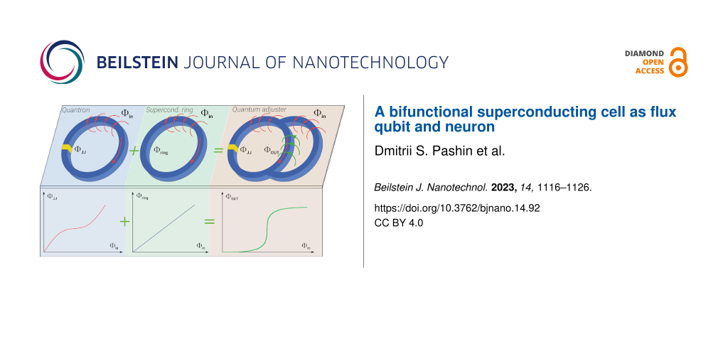
Apparently, the simplest superconducting circuit with a nonlinear flux-to-flux transformation in the classical regime is a single-contact interferometer, as depicted in the left part of Figure 1. However, the typical form of the function f for such an element does not meet the aforementioned requirements. In the classical mode, it can be demonstrated [28] that the desired form of f(Φin) can be achieved by adding an inductance with a specially chosen linear flux-to-flux transformation to the interferometer, as illustrated in the right part of Figure 1. At zero temperature and under quasi-adiabatic changes in the circuit’s inputs, the desired transformation (now for average values) will occur even in the quantum regime, when the spectrum of eigenvalues of the system’s Hamiltonian operator is discrete. Nevertheless, it raises the question of how the proposed adjustment circuit will operate at finite (millikelvin) temperatures in the quantum regime and under the influence of relatively fast magnetic field control pulses? Will the tuning, coupling, and neromorphic co-processing circuits acquire new useful properties in the quantum regime?
![[2190-4286-14-92-1]](/bjnano/content/figures/2190-4286-14-92-1.png?scale=2.0&max-width=1024&background=FFFFFF)
Figure 1: The idea behind the creation of the bifunctional cell. The combination of a quantum interferometer (quantron) and a simple superconducting ring leads to the emergence of a parametron with a sigma-like transfer function. Φin(t) and Φout(t) are the normalised fluxes at the input and output of the circuit; ΦJJ(t) and Φring(t) correspond to the superconducting phase drops at Josephson heterostructure and superconducting inductor, respectively. Nota bene, such a transfer characteristic is a good activation function for a neuron in a perceptron-type network, suitable for primary signal processing for quantum computing systems.
Figure 1: The idea behind the creation of the bifunctional cell. The combination of a quantum interferometer ...
This article is devoted to the search for answers to these questions. Hence, below we explore the quantum dynamics of observables in superconducting interferometers, discuss the implications for quantum computing, and the challenges that remain to be addressed. In addition, we note the potential for utilising the findings to develop components of neuromorphic co-processors that collaborate with quantum computing systems. We will refer to the corresponding cell (a single-contact interferometer shunted by an inductance as depicted in Figure 1) further in the text as the “parametron”.
Model of the Proposed Bifunctional Cell
In this and subsequent sections, we consider a parametric quantron (parametron) under the influence of unipolar pulses of external magnetic flux. It should be noted that this system has proven to be a basic element of neural networks such as the perceptron with a sigmoidal input-to-output transformation function (sigma-neuron). Preliminary calculations have shown that under certain conditions, such a neuron can operate successfully in both classical and quantum modes [24,26,28,30]. The energy of the system in the Hamiltonian formalism can be expressed as follows:
![[2190-4286-14-92-i1]](/bjnano/content/inline/2190-4286-14-92-i1.svg?max-width=590&scale=1.18182)
where the coefficients a and b are defined by the following expressions [28,30]:
![[2190-4286-14-92-i2]](/bjnano/content/inline/2190-4286-14-92-i2.svg?max-width=590&scale=1.18182)
Here, l is the normalised inductance of the quantron part of the sigma-interferometer (l = 2πLIc/Φ0), la is the additional linear inductance, and lout is the output inductance (la and lout are normalised in the same manner as l). Here and further, we use magnetic fluxes normalised by the quantum value, Φ0.
To investigate the flux-to-flux transfer characteristics of such a system, it is convenient to interpret its evolution as the movement of a particle with “mass” M = ![[Graphic 1]](/bjnano/content/inline/2190-4286-14-92-i21.svg?max-width=637&scale=1.18182) and “momentum” p =
and “momentum” p = ![[Graphic 2]](/bjnano/content/inline/2190-4286-14-92-i22.svg?max-width=637&scale=1.18182) in the potential profile defined by the second term in Equation 1, wherein the effective coordinate is a phase of the Josephson junction, φ. The quantities Ec =
in the potential profile defined by the second term in Equation 1, wherein the effective coordinate is a phase of the Josephson junction, φ. The quantities Ec = ![[Graphic 3]](/bjnano/content/inline/2190-4286-14-92-i23.svg?max-width=637&scale=1.18182) and EJ =
and EJ = ![[Graphic 4]](/bjnano/content/inline/2190-4286-14-92-i24.svg?max-width=637&scale=1.18182) are the capacitive and the Josephson energy, respectively, determined by critical current Ic and the capacity C of the Josephson junction. A typical example of “flux-based” system state management is provided by the dynamically varying input magnetic flux:
are the capacitive and the Josephson energy, respectively, determined by critical current Ic and the capacity C of the Josephson junction. A typical example of “flux-based” system state management is provided by the dynamically varying input magnetic flux:
![[2190-4286-14-92-i3]](/bjnano/content/inline/2190-4286-14-92-i3.svg?max-width=590&scale=1.18182)
This flux pulse is characterised by the level A, rise/fall rate of the signal DR/F, and the characteristic times t1 and t2 = 3t1 responsible for the rise and fall periods of the input magnetic flux. It is assumed that the time is given in units of ![[Graphic 5]](/bjnano/content/inline/2190-4286-14-92-i25.svg?max-width=637&scale=1.18182) , where
, where ![[Graphic 6]](/bjnano/content/inline/2190-4286-14-92-i26.svg?max-width=637&scale=1.18182) .
.
In the framework of the adiabatic approach, one can numerically find “instantaneous” energy levels En(t) and “instantaneous” eigenfunctions |ψn(t)⟩ of the system solving the stationary Schrödinger equation using the finite difference method [35]:
![[2190-4286-14-92-i4]](/bjnano/content/inline/2190-4286-14-92-i4.svg?max-width=590&scale=1.18182)
If at each moment in time, the state energy En(t) is much smaller than the distance between energy levels in the system, then the adiabatic approximation is valid and, therefore, transitions between instantaneous eigenstates can be neglected. Mathematically this condition can be expressed as:
![[2190-4286-14-92-i5]](/bjnano/content/inline/2190-4286-14-92-i5.svg?max-width=590&scale=1.18182)
which just defines the standard Landau–Zener problem [36-38]. If the adiabatic approximation is violated, for example, when the energy levels En(t) and Em(t) converge (anticrossing), Landau–Zener transitions occur. The rate of these transitions is controlled by the form of the external influence. At moments of level convergence for short periods τLZ, the phases of the wave functions change significantly, leading to strong fluctuations of the level populations in the system, and can lead to quasi-random dynamics in the parametron. In addition, Landau–Zener interference has become a tool to access the multilevel structure of these artificial atoms [39-42]. It is also used to obtain information about the connection of the qubits with a noisy environment and to form dissipative stable entanglements in quantum tomography protocols [43-45]. Let us further consider the limitations that such non-adiabatic effects impose on the potential use of the proposed cell as a neuromorphic, coupling, and tuning element in quantum computing systems. At the same time, we will also gain an understanding of the possibilities for controlling the population of levels in the simplest implementation of an adiabatic superconducting logic cell when used as an auxiliary qubit.
A Bifunctional Superconducting Cell as a Controllable Flux Qubit
The state dynamics of the considered system equation (Equation 1) are primarily defined by features of the controlling field equation (Equation 3), as well as by the values of the inductances. We have considered two cases of external field influence to the system, namely (i) when the controlling field has symmetrical rise/fall fronts, DR = DF = D, and (ii) when it does not, DR ≠ DF. It is assumed that at the initial time, the system is initialised to the ground state, that is, localised at the level with energy E0. The evolution of energy level population and instantaneous energy levels was numerically calculated for the n = 10 lowest energy levels of the quantum interferometer. As shown in Figure 2a,b, during rise and fall of the field, the instantaneous energy levels are getting closer, and the anticrossing effect is observed. For the ground and first-excited states, characteristic times of anticrossing correspond to τLZ, when the adiabatic condition (Equation 5) is violated and a non-zero probability of Landau–Zener tunneling between these energy levels emerges. As long as the leakage to upper states (for n > 2) during such transitions is less than |P1 − P0| − Pn≥2 ≪ |P1 − P0|, the two-levels approximation (n = 2) can be applied for analytical estimations of Landau–Zener transition probabilities [39,42]. Within this approximation, the system can be approximated by the following Hamiltonian:
![[2190-4286-14-92-i6]](/bjnano/content/inline/2190-4286-14-92-i6.svg?max-width=590&scale=1.18182)
where Δ = E1(tLZ) − E0(tLZ) determines the distance between energy levels at the moment of their closest convergence, and ε(τLZ) determines the type of levels anticrossing. The instantaneous energy levels of the ground and excited states can then be written as E0,1(τLZ) = ![[Graphic 7]](/bjnano/content/inline/2190-4286-14-92-i27.svg?max-width=637&scale=1.18182) .
.
![[2190-4286-14-92-2]](/bjnano/content/figures/2190-4286-14-92-2.png?scale=2.0&max-width=1024&background=FFFFFF)
Figure 2: (a, b) Time-dependence of the populations of ground state, P0(t), (black curve) and first excited state, P1(t), (red curve). Additionally, the four lowest states Ei(t) of the quantum interferometer are also demonstrated for (a) l = 2.63 and D = 0.0044 and (b) l = 2.69, DR = 0.008 and DF = 0.002. Diabatic levels for E0,1 are shown in the insert by the dashed line, and analytical estimations in the two-level approximation (from Equation 10) are shown by dots. (c, d) Interference population map for the first excited state for various values of the inductance l and rates of change of the control field fronts DR/F. The white dashed line denotes the violation boundary of the adiabatic approximation according to Equation 12 with accuracy equal to PLZ > 1%. For D = 0.0044 (e) and DR = 0.008 and DF = 0.002 (f), cross sections of probabilities P1(l) are given, which are marked with red arrows in (c, d). (g, h) Population of the excited state as a function of Δt = t2 − t1 with fixed values of (a) l = 2.63 and (b) l = 2.69 at the end of external influence. The plots in (a, c, e, g) were calculated for a symmetrical φin(t), while the plots in (b, d, f, h) were calculated for an asymmetrical input flux. The parameters of the system were la = 1 + l, lout = 0.1, EJ = 2Ec, and t1 = 3t2.
Figure 2: (a, b) Time-dependence of the populations of ground state, P0(t), (black curve) and first excited s...
Let us estimate the Landau–Zener transition probability at the moment of the first levels’ convergence, which corresponds to the time tLZ for diabatic dynamics (when Δ → 0) of level crossing (dashed lines in inserts in Figure 2a,b). As clearly seen from the simulation, the anticrossing effect occurs on small time scales near the moment of convergence tLZ. This allows us to use a linear approximation on time ε(tLZ + τLZ) ≈ ε′(tLZ)·τLZ and write the Hamiltonian of the system as:
![[2190-4286-14-92-i7]](/bjnano/content/inline/2190-4286-14-92-i7.svg?max-width=590&scale=1.18182)
We assume that V(τLZ) = ![[Graphic 8]](/bjnano/content/inline/2190-4286-14-92-i28.svg?max-width=637&scale=1.18182) is small on the scale of the Landau–Zener transition time. This allows us to use the perturbation theory to estimate the value of ε′(tLZ). In the moment of anticrossing, instantaneous energy levels E0 and E1 reach their extremum. Therefore, it is necessary to take into consideration the second order of perturbation theory for an analytical estimation of the convergence value:
is small on the scale of the Landau–Zener transition time. This allows us to use the perturbation theory to estimate the value of ε′(tLZ). In the moment of anticrossing, instantaneous energy levels E0 and E1 reach their extremum. Therefore, it is necessary to take into consideration the second order of perturbation theory for an analytical estimation of the convergence value:
![[2190-4286-14-92-i8]](/bjnano/content/inline/2190-4286-14-92-i8.svg?max-width=590&scale=1.18182)
where V01(τLZ) ≡ ⟨ψ0(tLZ)|V(τLZ)|ψ1(tLZ)⟩. Finally, from Equation 8 the difference between the energy levels is
![[2190-4286-14-92-i9]](/bjnano/content/inline/2190-4286-14-92-i9.svg?max-width=590&scale=1.18182)
Expanding the row up to the second order, we can get the difference between the levels:
![[2190-4286-14-92-i10]](/bjnano/content/inline/2190-4286-14-92-i10.svg?max-width=590&scale=1.18182)
Then, from Equation 9 and Equation 10, we obtain:
![[2190-4286-14-92-i11]](/bjnano/content/inline/2190-4286-14-92-i11.svg?max-width=590&scale=1.18182)
The dots in the insets to Figure 2a,b show the behaviour of the adiabatic energy levels at anticrossing τLZ. The estimates obtained in the framework of the two-level model are in good agreement with the numerical calculations (solid lines in Figure 2a,b) of the Schrödinger time-dependent equation by the Crank–Nicolson method [46] based on the Magnus decomposition for the evolutionary operator up to the fourth order. This agreement indicates the correctness of the approximations used for the estimation. Based on the resulting expression for the linear coefficient expression (Equation 11) for ε(tLZ + τLZ), we use the well-known formula for calculating the probability of Landau–Zener transitions [39,42] with a single convergence of the levels:
![[2190-4286-14-92-i12]](/bjnano/content/inline/2190-4286-14-92-i12.svg?max-width=590&scale=1.18182)
Using the obtained formula (Equation 12), we estimate the limit of occurrence of Landau–Zener transitions for different parameters of the control field and inductances in the circuit. To do this, we calculated the interference probability maps of the populations of the first excited level for typical quantum well inductances l and different parameters DR,F for symmetric (Figure 2c) and asymmetric (Figure 2d) external control fields at the time corresponding to the end of the external influence. Bright areas in Figure 2c,d correspond to regions where there is a non-zero probability of quantum-coherent Landau–Zener tunneling, and black areas correspond to the adiabatic control of the system. According to the expressions in Equation 12, the white dashed line in Figure 2c denotes the limit of the transition probability from the ground to the excited state PLZ < 0.01. This estimate is important for evaluating the functioning of this circuit in adiabatic quantum neural networks, where there are strict requirements for the absence of excitation from the initial state for the implementation of sigmoidal activation functions [30].
We can see from Figure 2e that for the symmetric control field for given DR,F, there are ranges of inductance values l where we can control the populations of levels by external influence using the Landau–Zener tunneling effect. In other words, in this parameter range we can, if necessary, control the state of the simplest adiabatic cell used as an auxiliary qubit. This parameter range is also important for the observation of quantum non-perturbative effects for the parametron that acts as a nonlinear adjuster, implementing the interaction between fluxonium type qubits [47,48]. In the case of an asymmetric control field, see Figure 2f, there is no complete transition between the E0 and E1 states in the system for a wide range of inductances, indicating the practical expediency of using a symmetric control influence. Another way of controlling the change in the level populations in the system is to control the phase difference between a pair of converging levels in the regions of increase (or decrease) in the external field, which of course depends on Δt = t2 − t1. These dependencies are naturally periodic, as shown in Figure 2g,h, for the two cases of application of an external field.
The action time of the symmetric input flux to avoid Landau–Zener transitions is ∼100 ns for l = 2. The estimate was made with the characteristic parameters of a Josephson junction, that is, Ic = 50 nA and C = 6 fF. In contrast, it takes ∼30 ns for the transition from the ground state to the first excited state, as shown in Figure 2a. It can be assumed that the characteristic duration of the “NOT” operation will be of the same order of magnitude for the “flux control” of the tuning circuit cell used as an auxiliary qubit.
A Model for Dissipative Effects in the Bifunctional Cell
Another important aspect to consider is the investigation of the impact of dissipative and temperature effects on the nonlinear dynamics of quantum interferometers. Quantum noise can result in the breakdown of coherence in the system and affect the operation of the parametron within coupling circuits and tuning schemes. In order to accurately describe these processes, we present the complete Hamiltonian of the system as:
![[2190-4286-14-92-i13]](/bjnano/content/inline/2190-4286-14-92-i13.svg?max-width=590&scale=1.18182)
where Hsys(t) is defined by Equation 1, and HR is the energy of the thermal bosonic reservoir of the form:
![[2190-4286-14-92-i14]](/bjnano/content/inline/2190-4286-14-92-i14.svg?max-width=590&scale=1.18182)
where Ωi is the frequency of the i-th bosonic mode, and ![[Graphic 9]](/bjnano/content/inline/2190-4286-14-92-i29.svg?max-width=637&scale=1.18182) and bi are, respectively, creation and annihilation operators for the i-th bosonic mode. Hint is responsible for the interaction between the thermostat and the superconducting parametron. For the case of ohmic dissipation, this relationship is linear and can be written as:
and bi are, respectively, creation and annihilation operators for the i-th bosonic mode. Hint is responsible for the interaction between the thermostat and the superconducting parametron. For the case of ohmic dissipation, this relationship is linear and can be written as:
![[2190-4286-14-92-i15]](/bjnano/content/inline/2190-4286-14-92-i15.svg?max-width=590&scale=1.18182)
where k is a coupling constant.
Within the framework of the adiabatic approximation, we can form the density matrix of the system in the instantaneous basis |ψn(t)⟩ as
![[2190-4286-14-92-i16]](/bjnano/content/inline/2190-4286-14-92-i16.svg?max-width=590&scale=1.18182)
In the Born–Markov approximation, the dissipative dynamic of a quantum system is described by an adiabatic generalised equation for the density matrix [49]. In terms of the instantaneous basis in the Schrödinger representation, the dynamics of the parametron obey the Redfield equation:
![[2190-4286-14-92-i17]](/bjnano/content/inline/2190-4286-14-92-i17.svg?max-width=590&scale=1.18182)
with ![[Graphic 10]](/bjnano/content/inline/2190-4286-14-92-i30.svg?max-width=637&scale=1.18182) and Lnm = |ψn(t)⟩⟨ψm(t)|⟨ψn(t)|φ|ψm(t)⟩. Here, we do not take into account the Lamb shift;
and Lnm = |ψn(t)⟩⟨ψm(t)|⟨ψn(t)|φ|ψm(t)⟩. Here, we do not take into account the Lamb shift; ![[Graphic 11]](/bjnano/content/inline/2190-4286-14-92-i31.svg?max-width=637&scale=1.18182) is the renormalised coupling constant, where g is the density of bosonic modes, θ is the Heaviside function, and
is the renormalised coupling constant, where g is the density of bosonic modes, θ is the Heaviside function, and ![[Graphic 12]](/bjnano/content/inline/2190-4286-14-92-i32.svg?max-width=637&scale=1.18182) is the Planck distribution. Note that we believe that the renormalised coupling constant does not depend on the frequency of the bosonic mode. We also used a numerical solution of the Redfield equation based on the Fock representation [50] using supercomputer modeling tools to obtain the results.
is the Planck distribution. Note that we believe that the renormalised coupling constant does not depend on the frequency of the bosonic mode. We also used a numerical solution of the Redfield equation based on the Fock representation [50] using supercomputer modeling tools to obtain the results.
It should be noted that Equation 17 is valid under the standard adiabatic condition: h/δ2 ≪ 1, where ![[Graphic 13]](/bjnano/content/inline/2190-4286-14-92-i33.svg?max-width=637&scale=1.18182) and
and ![[Graphic 14]](/bjnano/content/inline/2190-4286-14-92-i34.svg?max-width=637&scale=1.18182) The ratio h/δ2 ≈ 0.08 for the characteristic parameters l = 2 and D = 0.001.
The ratio h/δ2 ≈ 0.08 for the characteristic parameters l = 2 and D = 0.001.
We will apply the described model to analyse the limitations on the operating temperature range when using the proposed parametron in coupling circuits and tuning schemes in quantum computing systems.
A Bifunctional Superconducting Cell as an Adiabatic Neuron
The analysis conducted in section “A Bifunctional Superconducting Cell as a Controllable Flux Qubit” showed that Landau–Zener transitions significantly affect the dynamics of the system. Even in the case of adiabatic control, relaxation and thermal excitation processes can introduce additional difficulties that need to be considered when designing quantum interferometers and tuning circuits, adjusters, and neurons based on them. In particular, dissipative processes significantly affect the flux-to-flux transfer characteristics of such systems. In [30], we demonstrated that increasing the coupling coefficient of the interferometer with the reservoir suppresses oscillations of the mean flux value (generalised coordinate) caused by nonadiabatic interference effects. However, another important factor (in addition to relaxation) that influences the evolution of observable quantities for an interferometer is thermal fluctuations. It is known that the operating temperature, T, of quantum circuits with Josephson junctions is chosen much smaller than the characteristic temperature scale given by the distance between their ground and first excited energy levels:
![[2190-4286-14-92-i18]](/bjnano/content/inline/2190-4286-14-92-i18.svg?max-width=590&scale=1.18182)
At the same time, the probability of reaching higher energy levels is proportional to
![[Graphic 15]](/bjnano/content/inline/2190-4286-14-92-i35.svg?max-width=637&scale=1.18182)
and the distance between the instantaneous energy levels depends on the applied external control field φin(t), see Figure 3a. For example, for the parameters l = 2 and D = 0.001, corresponding to the adiabatic control region with symmetric magnetic flux (see Figure 2c), the energy gap between ground and first excited states attains its minimum value equal to ![[Graphic 16]](/bjnano/content/inline/2190-4286-14-92-i36.svg?max-width=637&scale=1.18182) during increase and decrease of the external flux (the common form of the dependence is shown in Figure 3b). During these time intervals, the condition in Equation 18 may be violated, leading to transitions to higher energy levels. Therefore, an analysis of the parameter behaviour as a function of the working temperature is required to find operating modes where the probability of such thermal transitions is minimised.
during increase and decrease of the external flux (the common form of the dependence is shown in Figure 3b). During these time intervals, the condition in Equation 18 may be violated, leading to transitions to higher energy levels. Therefore, an analysis of the parameter behaviour as a function of the working temperature is required to find operating modes where the probability of such thermal transitions is minimised.
![[2190-4286-14-92-3]](/bjnano/content/figures/2190-4286-14-92-3.png?scale=2.0&max-width=1024&background=FFFFFF)
Figure 3: (a) The spectrum of the Hamiltonian (Equation 1) as a function of the external flux φin(t) based on the numerical finite difference method [35]. (b) Blue solid line: temporal dependence of the distance between the ground state, E0(t), and the first excited state, E1(t), in the instantaneous basis of the parametron in quantum regime. Black dashed line: dependence of the input magnetic flux φin on time. The parameters of the circuit are l = 2, D = 0.001, A = 4π, la = 1 + l, lout = 0.1, EJ = 2Ec, t1 = 4000, and t1 = 3t2.
Figure 3: (a) The spectrum of the Hamiltonian (Equation 1) as a function of the external flux φin(t) based on the numer...
We focused our attention on macroscopic observables in the parametron in the quantum regime, such as the transfer characteristic iout = f(φin). For the considered scheme shown in Figure 1, this dependence can be expressed through the following relation:
![[2190-4286-14-92-i19]](/bjnano/content/inline/2190-4286-14-92-i19.svg?max-width=590&scale=1.18182)
Here, ⟨i⟩ = bφin(t) − a⟨φ⟩ is the mean value of the current operator on the Josephson junction when the external flux changes relative to the mean phase of the contact ⟨φ⟩ = ⟨ψ(t)|φ|ψ(t)⟩. As shown in Figure 4a, the transfer characteristic of the parametron has a sigmoidal dependence. It is worth noting that this feature allows for the use of the proposed scheme in superconducting neural networks, such as perceptrons, integrated into hybrid quantum-neuromorphic computers. Moreover, the temperature affects the steepness of the sigmoid function. Even the manifestation of hysteresis in flux-to-flux transformations (when iout(φin) during the increase of the external signal φin = 0 ![[Graphic 17]](/bjnano/content/inline/2190-4286-14-92-i37.svg?max-width=637&scale=1.18182) φin = A, solid lines in Figure 4a, does not coincide with the behaviour of the mean values during the decrease of the magnetic signal φin = A
φin = A, solid lines in Figure 4a, does not coincide with the behaviour of the mean values during the decrease of the magnetic signal φin = A ![[Graphic 18]](/bjnano/content/inline/2190-4286-14-92-i38.svg?max-width=637&scale=1.18182) φin = 0, dashed lines in Figure 4a). We also emphasise that the sigmoidal transfer characteristic obtained is very useful for using the adiabatic cell in question as an auxiliary qubit. This feature of the system’s behaviour, together with the possibility of tuning the energy spectrum, makes it possible to minimise its parasitic “magnetic” influence on the environment.
φin = 0, dashed lines in Figure 4a). We also emphasise that the sigmoidal transfer characteristic obtained is very useful for using the adiabatic cell in question as an auxiliary qubit. This feature of the system’s behaviour, together with the possibility of tuning the energy spectrum, makes it possible to minimise its parasitic “magnetic” influence on the environment.
![[2190-4286-14-92-4]](/bjnano/content/figures/2190-4286-14-92-4.png?scale=2.0&max-width=1024&background=FFFFFF)
Figure 4:
(a) Influence of temperature on the transfer characteristic of the parametron in the quantum regime. The solid lines represent the “forward” evolution of the system (φin = 0 ![[Graphic 19]](/bjnano/content/inline/2190-4286-14-92-i39.svg?max-width=637&scale=1.18182) φin = A), and the dashed lines represent the “reverse” evolution (φin = A
φin = A), and the dashed lines represent the “reverse” evolution (φin = A ![[Graphic 20]](/bjnano/content/inline/2190-4286-14-92-i40.svg?max-width=637&scale=1.18182) φin = 0). The black curve corresponds to the zero-temperature case, while the blue and red curves correspond to temperatures of 0.5 and 1 K, respectively. (b) The region of parameters where the transfer characteristic is close to a sigmoidal shape with a standard deviation of SD < 10−4. In the white area, even at zero temperature, the standard deviation is larger then SD = 10−4. The system parameters used in the simulation were A = 4π, a coupling coefficient with the thermostat determined by condition κ = 0.0025ωp, la = 1 + l, lout = 0.1, EJ = 2Ec, and t1 = 3t2.
φin = 0). The black curve corresponds to the zero-temperature case, while the blue and red curves correspond to temperatures of 0.5 and 1 K, respectively. (b) The region of parameters where the transfer characteristic is close to a sigmoidal shape with a standard deviation of SD < 10−4. In the white area, even at zero temperature, the standard deviation is larger then SD = 10−4. The system parameters used in the simulation were A = 4π, a coupling coefficient with the thermostat determined by condition κ = 0.0025ωp, la = 1 + l, lout = 0.1, EJ = 2Ec, and t1 = 3t2.
Figure 4: (a) Influence of temperature on the transfer characteristic of the parametron in the quantum regime...
Figure 4b presents the temperature map showing the maximum temperature at which the transfer characteristic of the parametron is sufficiently close to a sigmoid. To construct this map, we considered curves for which the standard deviation, SD, from the mathematical sigmoid did not exceed 10−4. The ordinate and abscissa axes correspond to the rise/fall rates of the applied flux and the normalised inductance of the cell, respectively. The calculations show that as the inductance of the parametron l and the performance of it increases, the requirements for system temperature control also increase, necessitating increasingly lower operating temperatures. For example, the dark blue region in Figure 4b is only suitable for T ∼ 0.1 K. Note that for the parameters used and a Josephson junction quality factor of Q ∼ 105, the relaxation time is tr ∼ 1 μs. From this rough estimate it can be seen that in the future, adiabatic cells of tuning circuits can also be used as auxiliary qubits for a more efficient use of structures on a “quantum” chip.
Results and Discussion
We have already considered the system presented in the article in our previous work [30]. But we considered it exclusively as a classical adiabatic neural network cell, even when we studied its dynamics in the quantum mode. The main result of this work is to demonstrate a good quantum logic operation with a relatively short duration on a single-contact inductively shunted interferometer (see Figure 2). After all, such a system has not been considered commonly by the modern scientific community to be a good flux qubit. We were also surprised by the possibility of controlling the qubit state using unipolar current pulses, which greatly simplifies all control electronics [51,52]. But won’t such a deliberately non-resonant (broadband) impact lead to a parasitic leakage of the state to higher levels? We have conducted a separate study of this issue, the results of which are presented in this section.
The amount of leakage from the computational qubit basis when implementing a good “NOT” operation is mainly influenced by (i) the distance between the converging energy levels, Δt = t2 − t1, and (ii) the rise/fall rate of the control pulse DR,F. At the same time, a fairly significant range of acceptable parameters is highlighted (the light colour in Figure 5a) when the “NOT” operation is implemented in the system via Landau–Zener transitions. Usually, this “working” range of parameters varies from l = 2.2 for D = 0.008 up to l = 2.7 for D = 0.0035, which gives an estimated duration of the operation of 20–60 ns (for the selected typical parameters of the Josephson contact, Ic = 50 nA and C = 6 fF). Furthermore, in order to assess the quality of this operation and to control the leakage into the overlying states in Figure 5b, we show the behaviour of the population of the second excited level, P2, in the system for various values of D and l. The leakage into the second state is dominant (see Figure 5c). The oscillations on the curves are due to a more complex double anticrossing (in the case of leakage to P2, the blue curve in Figure 5c, this is the convergence of the first and second levels) and the acquired progression of Stuckelberg phases. Similar behaviour was also found for different initial states of the qubit, Figure 5d. We have evaluated the reliability of such an operation based on the calculation of fidelity. We evaluate the fidelity of the gate Ug (for Figure 2a) as in [53]:
![[2190-4286-14-92-i20]](/bjnano/content/inline/2190-4286-14-92-i20.svg?max-width=590&scale=1.18182)
where the summation runs over the six states ν aligned along the cardinal directions of the Bloch sphere ![[Graphic 21]](/bjnano/content/inline/2190-4286-14-92-i41.svg?max-width=637&scale=1.18182)
![[Graphic 22]](/bjnano/content/inline/2190-4286-14-92-i42.svg?max-width=637&scale=1.18182) |z+⟩ = |0⟩, |z−⟩ = |1⟩. Here, |0⟩ and |1⟩ are the ground and first excited states of the system, and Uid is the matrix of an ideal qubit gate. For the “NOT” operation shown in Figure 2a for l = 2.63 and D = 0.0044, taking into account the optimisation of the pulse parameters Δt, according to Figure 2g and Figure 5, we can get the fidelity of the operation F = 99.99%. We can therefore say with confidence that the same cell can be used both as a classical adiabatic neuron and as a qubit whose state can be controlled with an infidelity of the order of 0.0001.
|z+⟩ = |0⟩, |z−⟩ = |1⟩. Here, |0⟩ and |1⟩ are the ground and first excited states of the system, and Uid is the matrix of an ideal qubit gate. For the “NOT” operation shown in Figure 2a for l = 2.63 and D = 0.0044, taking into account the optimisation of the pulse parameters Δt, according to Figure 2g and Figure 5, we can get the fidelity of the operation F = 99.99%. We can therefore say with confidence that the same cell can be used both as a classical adiabatic neuron and as a qubit whose state can be controlled with an infidelity of the order of 0.0001.
![[2190-4286-14-92-5]](/bjnano/content/figures/2190-4286-14-92-5.png?scale=2.0&max-width=1024&background=FFFFFF)
Figure 5: Interference population map for the first excited state (a) and the second state (b) for different values of the inductance l and rates of change of the control field fronts D. (c) Time-dependent dynamics of the overlying states (n = 2, 3, 4) and (d) leakage to the second excited level (n = 2) for the system initialised at different poles on the Bloch sphere for the values l = 2.63 and D = 0.0044, similar to those shown in Figure 2a. The parameters of the system were la = 1 + l, lout = 0.1, EJ = 2Ec, and t1 = 3t2.
Figure 5: Interference population map for the first excited state (a) and the second state (b) for different ...
Conclusion
The simplest cell of adiabatic superconducting logic can function even in quantum mode as an element of tuning circuits if the control signals change quasi-adiabatically with time (rise/fall times for control fields are more than a 100 ns). At sufficiently low temperatures and relatively small normalised inductances, such an inductively shunted single-contact interferometer can also be used as part of a perceptron-type neural network to process signals received from qubits. Such a cell can be used in quantum mode also as an auxiliary qubit with relatively fast “flux” control. Future research will address the problem of using more advanced adiabatic superconducting logic cells for such purposes. In addition, bifunctional cells, which can act as adiabatic neurons or flux qubits depending on the operating conditions, have the potential to be used to simulate the operations in a non-classical brain [54,55].
Funding
The development of the method of analysing the evolution of observables for the adiabatic logic cells in quantum mode was carried out with the support of the Grant of the Russian Science Foundation No. 22-72-10075. The development of the main concept was carried out with the financial support of the Strategic Academic Leadership Programme “Priority-2030” (grant from NITU “MISIS” No. K2-2022-029). A.S. is grateful to the Foundation for the Advancement of Theoretical Physics and Mathematics “BASIS” (grant 22-1-3-16-1).
References
-
Dattani, N.; Szalay, S.; Chancellor, N. arXiv 2019, No. 1901.07636.
Return to citation in text: [1] -
Vyskocil, T.; Djidjev, H. Algorithms 2019, 12, 77. doi:10.3390/a12040077
Return to citation in text: [1] -
Boothby, K.; Bunyk, P.; Raymond, J.; Roy, A. arXiv 2020, No. 2003.00133.
Return to citation in text: [1] -
Boothby, K.; King, A. D.; Raymond, J. Zephyr Topology of D-Wave Quantum Processors; D-Wave Technical Report Series; D-Wave Systems Inc., 2021.
Return to citation in text: [1] -
Manucharyan, V. E.; Koch, J.; Glazman, L. I.; Devoret, M. H. Science 2009, 326, 113–116. doi:10.1126/science.1175552
Return to citation in text: [1] -
Nguyen, L. B.; Lin, Y.-H.; Somoroff, A.; Mencia, R.; Grabon, N.; Manucharyan, V. E. Phys. Rev. X 2019, 9, 041041. doi:10.1103/physrevx.9.041041
Return to citation in text: [1] -
Grover, J. A.; Basham, J. I.; Marakov, A.; Disseler, S. M.; Hinkey, R. T.; Khalil, M.; Stegen, Z. A.; Chamberlin, T.; DeGottardi, W.; Clarke, D. J.; Medford, J. R.; Strand, J. D.; Stoutimore, M. J. A.; Novikov, S.; Ferguson, D. G.; Lidar, D.; Zick, K. M.; Przybysz, A. J. PRX Quantum 2020, 1, 020314. doi:10.1103/prxquantum.1.020314
Return to citation in text: [1] -
Zhang, H.; Chakram, S.; Roy, T.; Earnest, N.; Lu, Y.; Huang, Z.; Weiss, D. K.; Koch, J.; Schuster, D. I. Phys. Rev. X 2021, 11, 011010. doi:10.1103/physrevx.11.011010
Return to citation in text: [1] -
Gyenis, A.; Mundada, P. S.; Di Paolo, A.; Hazard, T. M.; You, X.; Schuster, D. I.; Koch, J.; Blais, A.; Houck, A. A. PRX Quantum 2021, 2, 010339. doi:10.1103/prxquantum.2.010339
Return to citation in text: [1] -
Somoroff, A.; Ficheux, Q.; Mencia, R. A.; Xiong, H.; Kuzmin, R.; Manucharyan, V. E. Phys. Rev. Lett. 2023, 130, 267001. doi:10.1103/physrevlett.130.267001
Return to citation in text: [1] -
Takeuchi, N.; Ozawa, D.; Yamanashi, Y.; Yoshikawa, N. Supercond. Sci. Technol. 2013, 26, 035010. doi:10.1088/0953-2048/26/3/035010
Return to citation in text: [1] -
Takeuchi, N.; Yamanashi, Y.; Yoshikawa, N. Appl. Phys. Lett. 2013, 102, 052602. doi:10.1063/1.4790276
Return to citation in text: [1] -
Takeuchi, N.; Yamanashi, Y.; Yoshikawa, N. Appl. Phys. Lett. 2013, 103, 062602. doi:10.1063/1.4817974
Return to citation in text: [1] -
Takeuchi, N.; Yamanashi, Y.; Yoshikawa, N. Sci. Rep. 2014, 4, 6354. doi:10.1038/srep06354
Return to citation in text: [1] -
He, Y.; Takeuchi, N.; Yoshikawa, N. Appl. Phys. Lett. 2020, 116, 182602. doi:10.1063/5.0005612
Return to citation in text: [1] -
Ayala, C. L.; Tanaka, T.; Saito, R.; Nozoe, M.; Takeuchi, N.; Yoshikawa, N. IEEE J. Solid-State Circuits 2021, 56, 1152–1165. doi:10.1109/jssc.2020.3041338
Return to citation in text: [1] -
Takeuchi, N.; Yamae, T.; Ayala, C. L.; Suzuki, H.; Yoshikawa, N. IEICE Trans. Electron. 2022, E105.C, 251–263. doi:10.1587/transele.2021sep0003
Return to citation in text: [1] -
Schneider, M. L.; Donnelly, C. A.; Russek, S. E.; Baek, B.; Pufall, M. R.; Hopkins, P. F.; Dresselhaus, P. D.; Benz, S. P.; Rippard, W. H. Sci. Adv. 2018, 4, e1701329. doi:10.1126/sciadv.1701329
Return to citation in text: [1] -
Zhang, H.; Gang, C.; Xu, C.; Gong, G.; Lu, H. IEEE Trans. Emerg. Top. Comput. Intell. 2023, 7, 271–277. doi:10.1109/tetci.2021.3089328
Return to citation in text: [1] -
Ishida, K.; Byun, I.; Nagaoka, I.; Fukumitsu, K.; Tanaka, M.; Kawakami, S.; Tanimoto, T.; Ono, T.; Kim, J.; Inoue, K. IEEE Micro 2021, 41, 19–26. doi:10.1109/mm.2021.3070488
Return to citation in text: [1] -
Chalkiadakis, D.; Hizanidis, J. Phys. Rev. E 2022, 106, 044206. doi:10.1103/physreve.106.044206
Return to citation in text: [1] -
Schegolev, A. E.; Klenov, N. V.; Gubochkin, G. I.; Kupriyanov, M. Y.; Soloviev, I. I. Nanomaterials 2023, 13, 2101. doi:10.3390/nano13142101
Return to citation in text: [1] -
Karamuftuoglu, M. A.; Bozbey, A.; Ozbayoglu, M. IEEE Trans. Appl. Supercond. 2023, 33, 1304608. doi:10.1109/tasc.2023.3295835
Return to citation in text: [1] -
Schegolev, A. E.; Klenov, N. V.; Soloviev, I. I.; Tereshonok, M. V. Beilstein J. Nanotechnol. 2016, 7, 1397–1403. doi:10.3762/bjnano.7.130
Return to citation in text: [1] [2] -
Soloviev, I. I.; Schegolev, A. E.; Klenov, N. V.; Bakurskiy, S. V.; Kupriyanov, M. Y.; Tereshonok, M. V.; Shadrin, A. V.; Stolyarov, V. S.; Golubov, A. A. J. Appl. Phys. 2018, 124, 152113. doi:10.1063/1.5042147
Return to citation in text: [1] -
Schegolev, A.; Klenov, N.; Soloviev, I.; Tereshonok, M. Supercond. Sci. Technol. 2021, 34, 015006. doi:10.1088/1361-6668/abc569
Return to citation in text: [1] [2] -
Bakurskiy, S.; Kupriyanov, M.; Klenov, N. V.; Soloviev, I.; Schegolev, A.; Morari, R.; Khaydukov, Y.; Sidorenko, A. S. Beilstein J. Nanotechnol. 2020, 11, 1336–1345. doi:10.3762/bjnano.11.118
Return to citation in text: [1] -
Bastrakova, M.; Gorchavkina, A.; Schegolev, A.; Klenov, N.; Soloviev, I.; Satanin, A.; Tereshonok, M. Symmetry 2021, 13, 1735. doi:10.3390/sym13091735
Return to citation in text: [1] [2] [3] [4] -
Schegolev, A. E.; Klenov, N. V.; Bakurskiy, S. V.; Soloviev, I. I.; Kupriyanov, M. Y.; Tereshonok, M. V.; Sidorenko, A. S. Beilstein J. Nanotechnol. 2022, 13, 444–454. doi:10.3762/bjnano.13.37
Return to citation in text: [1] -
Bastrakova, M. V.; Pashin, D. S.; Rybin, D. A.; Schegolev, A. E.; Klenov, N. V.; Soloviev, I. I.; Gorchavkina, A. A.; Satanin, A. M. Beilstein J. Nanotechnol. 2022, 13, 653–665. doi:10.3762/bjnano.13.57
Return to citation in text: [1] [2] [3] [4] [5] [6] -
Islam, M. M.; Alam, S.; Hossain, M. S.; Roy, K.; Aziz, A. J. Appl. Phys. 2023, 133, 070701. doi:10.1063/5.0133515
Return to citation in text: [1] -
Li, Z.; Yuan, G.; Yamauchi, T.; Masoud, Z.; Xie, Y.; Dong, P.; Tang, X.; Yoshikawa, N.; Tiwari, D.; Wang, Y.; Chen, O. arXiv 2023, No. 2309.12212.
Return to citation in text: [1] -
Liu, Y.-x.; Wei, L. F.; Tsai, J. S.; Nori, F. Phys. Rev. Lett. 2006, 96, 067003. doi:10.1103/physrevlett.96.067003
Return to citation in text: [1] -
van der Ploeg, S. H. W.; Izmalkov, A.; van den Brink, A. M.; Hübner, U.; Grajcar, M.; Il’ichev, E.; Meyer, H.-G.; Zagoskin, A. M. Phys. Rev. Lett. 2007, 98, 057004. doi:10.1103/physrevlett.98.057004
Return to citation in text: [1] -
Press, W. H.; Teukolsky, S. A.; Vetterling, W. T.; Flannery, B. P. Numerical Recipes. The Art of Scientific Computing; Cambridge University Press: Cambridge, U.K., 2007.
Return to citation in text: [1] [2] -
Landau, L. D. Phys. Z. Sowjetunion 1932, 2, 46.
Return to citation in text: [1] -
Zener, C. Proc. R. Soc. London, Ser. A 1932, 137, 696–702. doi:10.1098/rspa.1932.0165
Return to citation in text: [1] -
Stückelberg, E. C. G. Helv. Phys. Acta 1932, 5, 369–423.
Return to citation in text: [1] -
Shevchenko, S. N.; Ashhab, S.; Nori, F. Phys. Rep. 2010, 492, 1–30. doi:10.1016/j.physrep.2010.03.002
Return to citation in text: [1] [2] [3] -
Mi, X.; Kohler, S.; Petta, J. R. Phys. Rev. B 2018, 98, 161404. doi:10.1103/physrevb.98.161404
Return to citation in text: [1] -
Satanin, A. M.; Denisenko, M. V.; Ashhab, S.; Nori, F. Phys. Rev. B 2012, 85, 184524. doi:10.1103/physrevb.85.184524
Return to citation in text: [1] -
Ivakhnenko, O. V.; Shevchenko, S. N.; Nori, F. Phys. Rep. 2023, 995, 1–89. doi:10.1016/j.physrep.2022.10.002
Return to citation in text: [1] [2] [3] -
Gramajo, A. L.; Domínguez, D.; Sánchez, M. J. Phys. Rev. A 2018, 98, 042337. doi:10.1103/physreva.98.042337
Return to citation in text: [1] -
Munyaev, V. O.; Bastrakova, M. V. Phys. Rev. A 2021, 104, 012613. doi:10.1103/physreva.104.012613
Return to citation in text: [1] -
Gramajo, A. L.; Domínguez, D.; Sánchez, M. J. Phys. Rev. A 2021, 104, 032410. doi:10.1103/physreva.104.032410
Return to citation in text: [1] -
Crank, J.; Nicolson, P. A practical method for numerical evaluation of solutions of partial differential equations of the heat-conduction type. In Mathematical proceedings of the Cambridge philosophical society, 1947; pp 50–67.
Return to citation in text: [1] -
Moskalenko, I. N.; Besedin, I. S.; Simakov, I. A.; Ustinov, A. V. Appl. Phys. Lett. 2021, 119, 194001. doi:10.1063/5.0064800
Return to citation in text: [1] -
Moskalenko, I. N.; Simakov, I. A.; Abramov, N. N.; Grigorev, A. A.; Moskalev, D. O.; Pishchimova, A. A.; Smirnov, N. S.; Zikiy, E. V.; Rodionov, I. A.; Besedin, I. S. npj Quantum Inf. 2022, 8, 130. doi:10.1038/s41534-022-00644-x
Return to citation in text: [1] -
Albash, T.; Boixo, S.; Lidar, D. A.; Zanardi, P. New J. Phys. 2012, 14, 123016. doi:10.1088/1367-2630/14/12/123016
Return to citation in text: [1] -
Pikunov, P. V.; Pashin, D. S.; Bastrakova, M. V. Numerical Simulation of Quantum Dissipative Dynamics of a Superconducting Neuron. In Mathematical Modeling and Supercomputer Technologies; Balandin, D.; Barkalov, K.; Meyerov, I., Eds.; Springer Nature Switzerland: Cham, 2022; pp 293–301. doi:10.1007/978-3-031-24145-1_24
Return to citation in text: [1] -
Bastrakova, M.; Klenov, N.; Ruzhickiy, V.; Soloviev, I.; Satanin, A. Supercond. Sci. Technol. 2022, 35, 055003. doi:10.1088/1361-6668/ac5505
Return to citation in text: [1] -
Caceres, J. J.; Dominguez, D.; Sanchez, M. J. arXiv 2023, No. 2309.00601.
Return to citation in text: [1] -
Bowdrey, M. D.; Oi, D. K. L.; Short, A. J.; Banaszek, K.; Jones, J. A. Phys. Lett. A 2002, 294, 258–260. doi:10.1016/s0375-9601(02)00069-5
Return to citation in text: [1] -
Kerskens, C. M.; López Pérez, D. J. Phys. Commun. 2022, 6, 105001. doi:10.1088/2399-6528/ac94be
Return to citation in text: [1] -
Widdows, D.; Rani, J.; Pothos, E. M. Entropy 2023, 25, 548. doi:10.3390/e25040548
Return to citation in text: [1]
| 1. | Dattani, N.; Szalay, S.; Chancellor, N. arXiv 2019, No. 1901.07636. |
| 2. | Vyskocil, T.; Djidjev, H. Algorithms 2019, 12, 77. doi:10.3390/a12040077 |
| 3. | Boothby, K.; Bunyk, P.; Raymond, J.; Roy, A. arXiv 2020, No. 2003.00133. |
| 4. | Boothby, K.; King, A. D.; Raymond, J. Zephyr Topology of D-Wave Quantum Processors; D-Wave Technical Report Series; D-Wave Systems Inc., 2021. |
| 5. | Manucharyan, V. E.; Koch, J.; Glazman, L. I.; Devoret, M. H. Science 2009, 326, 113–116. doi:10.1126/science.1175552 |
| 6. | Nguyen, L. B.; Lin, Y.-H.; Somoroff, A.; Mencia, R.; Grabon, N.; Manucharyan, V. E. Phys. Rev. X 2019, 9, 041041. doi:10.1103/physrevx.9.041041 |
| 7. | Grover, J. A.; Basham, J. I.; Marakov, A.; Disseler, S. M.; Hinkey, R. T.; Khalil, M.; Stegen, Z. A.; Chamberlin, T.; DeGottardi, W.; Clarke, D. J.; Medford, J. R.; Strand, J. D.; Stoutimore, M. J. A.; Novikov, S.; Ferguson, D. G.; Lidar, D.; Zick, K. M.; Przybysz, A. J. PRX Quantum 2020, 1, 020314. doi:10.1103/prxquantum.1.020314 |
| 8. | Zhang, H.; Chakram, S.; Roy, T.; Earnest, N.; Lu, Y.; Huang, Z.; Weiss, D. K.; Koch, J.; Schuster, D. I. Phys. Rev. X 2021, 11, 011010. doi:10.1103/physrevx.11.011010 |
| 9. | Gyenis, A.; Mundada, P. S.; Di Paolo, A.; Hazard, T. M.; You, X.; Schuster, D. I.; Koch, J.; Blais, A.; Houck, A. A. PRX Quantum 2021, 2, 010339. doi:10.1103/prxquantum.2.010339 |
| 10. | Somoroff, A.; Ficheux, Q.; Mencia, R. A.; Xiong, H.; Kuzmin, R.; Manucharyan, V. E. Phys. Rev. Lett. 2023, 130, 267001. doi:10.1103/physrevlett.130.267001 |
| 33. | Liu, Y.-x.; Wei, L. F.; Tsai, J. S.; Nori, F. Phys. Rev. Lett. 2006, 96, 067003. doi:10.1103/physrevlett.96.067003 |
| 34. | van der Ploeg, S. H. W.; Izmalkov, A.; van den Brink, A. M.; Hübner, U.; Grajcar, M.; Il’ichev, E.; Meyer, H.-G.; Zagoskin, A. M. Phys. Rev. Lett. 2007, 98, 057004. doi:10.1103/physrevlett.98.057004 |
| 39. | Shevchenko, S. N.; Ashhab, S.; Nori, F. Phys. Rep. 2010, 492, 1–30. doi:10.1016/j.physrep.2010.03.002 |
| 42. | Ivakhnenko, O. V.; Shevchenko, S. N.; Nori, F. Phys. Rep. 2023, 995, 1–89. doi:10.1016/j.physrep.2022.10.002 |
| 24. | Schegolev, A. E.; Klenov, N. V.; Soloviev, I. I.; Tereshonok, M. V. Beilstein J. Nanotechnol. 2016, 7, 1397–1403. doi:10.3762/bjnano.7.130 |
| 25. | Soloviev, I. I.; Schegolev, A. E.; Klenov, N. V.; Bakurskiy, S. V.; Kupriyanov, M. Y.; Tereshonok, M. V.; Shadrin, A. V.; Stolyarov, V. S.; Golubov, A. A. J. Appl. Phys. 2018, 124, 152113. doi:10.1063/1.5042147 |
| 26. | Schegolev, A.; Klenov, N.; Soloviev, I.; Tereshonok, M. Supercond. Sci. Technol. 2021, 34, 015006. doi:10.1088/1361-6668/abc569 |
| 27. | Bakurskiy, S.; Kupriyanov, M.; Klenov, N. V.; Soloviev, I.; Schegolev, A.; Morari, R.; Khaydukov, Y.; Sidorenko, A. S. Beilstein J. Nanotechnol. 2020, 11, 1336–1345. doi:10.3762/bjnano.11.118 |
| 28. | Bastrakova, M.; Gorchavkina, A.; Schegolev, A.; Klenov, N.; Soloviev, I.; Satanin, A.; Tereshonok, M. Symmetry 2021, 13, 1735. doi:10.3390/sym13091735 |
| 29. | Schegolev, A. E.; Klenov, N. V.; Bakurskiy, S. V.; Soloviev, I. I.; Kupriyanov, M. Y.; Tereshonok, M. V.; Sidorenko, A. S. Beilstein J. Nanotechnol. 2022, 13, 444–454. doi:10.3762/bjnano.13.37 |
| 30. | Bastrakova, M. V.; Pashin, D. S.; Rybin, D. A.; Schegolev, A. E.; Klenov, N. V.; Soloviev, I. I.; Gorchavkina, A. A.; Satanin, A. M. Beilstein J. Nanotechnol. 2022, 13, 653–665. doi:10.3762/bjnano.13.57 |
| 31. | Islam, M. M.; Alam, S.; Hossain, M. S.; Roy, K.; Aziz, A. J. Appl. Phys. 2023, 133, 070701. doi:10.1063/5.0133515 |
| 32. | Li, Z.; Yuan, G.; Yamauchi, T.; Masoud, Z.; Xie, Y.; Dong, P.; Tang, X.; Yoshikawa, N.; Tiwari, D.; Wang, Y.; Chen, O. arXiv 2023, No. 2309.12212. |
| 30. | Bastrakova, M. V.; Pashin, D. S.; Rybin, D. A.; Schegolev, A. E.; Klenov, N. V.; Soloviev, I. I.; Gorchavkina, A. A.; Satanin, A. M. Beilstein J. Nanotechnol. 2022, 13, 653–665. doi:10.3762/bjnano.13.57 |
| 18. | Schneider, M. L.; Donnelly, C. A.; Russek, S. E.; Baek, B.; Pufall, M. R.; Hopkins, P. F.; Dresselhaus, P. D.; Benz, S. P.; Rippard, W. H. Sci. Adv. 2018, 4, e1701329. doi:10.1126/sciadv.1701329 |
| 19. | Zhang, H.; Gang, C.; Xu, C.; Gong, G.; Lu, H. IEEE Trans. Emerg. Top. Comput. Intell. 2023, 7, 271–277. doi:10.1109/tetci.2021.3089328 |
| 20. | Ishida, K.; Byun, I.; Nagaoka, I.; Fukumitsu, K.; Tanaka, M.; Kawakami, S.; Tanimoto, T.; Ono, T.; Kim, J.; Inoue, K. IEEE Micro 2021, 41, 19–26. doi:10.1109/mm.2021.3070488 |
| 21. | Chalkiadakis, D.; Hizanidis, J. Phys. Rev. E 2022, 106, 044206. doi:10.1103/physreve.106.044206 |
| 22. | Schegolev, A. E.; Klenov, N. V.; Gubochkin, G. I.; Kupriyanov, M. Y.; Soloviev, I. I. Nanomaterials 2023, 13, 2101. doi:10.3390/nano13142101 |
| 23. | Karamuftuoglu, M. A.; Bozbey, A.; Ozbayoglu, M. IEEE Trans. Appl. Supercond. 2023, 33, 1304608. doi:10.1109/tasc.2023.3295835 |
| 39. | Shevchenko, S. N.; Ashhab, S.; Nori, F. Phys. Rep. 2010, 492, 1–30. doi:10.1016/j.physrep.2010.03.002 |
| 42. | Ivakhnenko, O. V.; Shevchenko, S. N.; Nori, F. Phys. Rep. 2023, 995, 1–89. doi:10.1016/j.physrep.2022.10.002 |
| 11. | Takeuchi, N.; Ozawa, D.; Yamanashi, Y.; Yoshikawa, N. Supercond. Sci. Technol. 2013, 26, 035010. doi:10.1088/0953-2048/26/3/035010 |
| 12. | Takeuchi, N.; Yamanashi, Y.; Yoshikawa, N. Appl. Phys. Lett. 2013, 102, 052602. doi:10.1063/1.4790276 |
| 13. | Takeuchi, N.; Yamanashi, Y.; Yoshikawa, N. Appl. Phys. Lett. 2013, 103, 062602. doi:10.1063/1.4817974 |
| 14. | Takeuchi, N.; Yamanashi, Y.; Yoshikawa, N. Sci. Rep. 2014, 4, 6354. doi:10.1038/srep06354 |
| 15. | He, Y.; Takeuchi, N.; Yoshikawa, N. Appl. Phys. Lett. 2020, 116, 182602. doi:10.1063/5.0005612 |
| 16. | Ayala, C. L.; Tanaka, T.; Saito, R.; Nozoe, M.; Takeuchi, N.; Yoshikawa, N. IEEE J. Solid-State Circuits 2021, 56, 1152–1165. doi:10.1109/jssc.2020.3041338 |
| 17. | Takeuchi, N.; Yamae, T.; Ayala, C. L.; Suzuki, H.; Yoshikawa, N. IEICE Trans. Electron. 2022, E105.C, 251–263. doi:10.1587/transele.2021sep0003 |
| 46. | Crank, J.; Nicolson, P. A practical method for numerical evaluation of solutions of partial differential equations of the heat-conduction type. In Mathematical proceedings of the Cambridge philosophical society, 1947; pp 50–67. |
| 35. | Press, W. H.; Teukolsky, S. A.; Vetterling, W. T.; Flannery, B. P. Numerical Recipes. The Art of Scientific Computing; Cambridge University Press: Cambridge, U.K., 2007. |
| 39. | Shevchenko, S. N.; Ashhab, S.; Nori, F. Phys. Rep. 2010, 492, 1–30. doi:10.1016/j.physrep.2010.03.002 |
| 40. | Mi, X.; Kohler, S.; Petta, J. R. Phys. Rev. B 2018, 98, 161404. doi:10.1103/physrevb.98.161404 |
| 41. | Satanin, A. M.; Denisenko, M. V.; Ashhab, S.; Nori, F. Phys. Rev. B 2012, 85, 184524. doi:10.1103/physrevb.85.184524 |
| 42. | Ivakhnenko, O. V.; Shevchenko, S. N.; Nori, F. Phys. Rep. 2023, 995, 1–89. doi:10.1016/j.physrep.2022.10.002 |
| 28. | Bastrakova, M.; Gorchavkina, A.; Schegolev, A.; Klenov, N.; Soloviev, I.; Satanin, A.; Tereshonok, M. Symmetry 2021, 13, 1735. doi:10.3390/sym13091735 |
| 30. | Bastrakova, M. V.; Pashin, D. S.; Rybin, D. A.; Schegolev, A. E.; Klenov, N. V.; Soloviev, I. I.; Gorchavkina, A. A.; Satanin, A. M. Beilstein J. Nanotechnol. 2022, 13, 653–665. doi:10.3762/bjnano.13.57 |
| 43. | Gramajo, A. L.; Domínguez, D.; Sánchez, M. J. Phys. Rev. A 2018, 98, 042337. doi:10.1103/physreva.98.042337 |
| 44. | Munyaev, V. O.; Bastrakova, M. V. Phys. Rev. A 2021, 104, 012613. doi:10.1103/physreva.104.012613 |
| 45. | Gramajo, A. L.; Domínguez, D.; Sánchez, M. J. Phys. Rev. A 2021, 104, 032410. doi:10.1103/physreva.104.032410 |
| 24. | Schegolev, A. E.; Klenov, N. V.; Soloviev, I. I.; Tereshonok, M. V. Beilstein J. Nanotechnol. 2016, 7, 1397–1403. doi:10.3762/bjnano.7.130 |
| 26. | Schegolev, A.; Klenov, N.; Soloviev, I.; Tereshonok, M. Supercond. Sci. Technol. 2021, 34, 015006. doi:10.1088/1361-6668/abc569 |
| 28. | Bastrakova, M.; Gorchavkina, A.; Schegolev, A.; Klenov, N.; Soloviev, I.; Satanin, A.; Tereshonok, M. Symmetry 2021, 13, 1735. doi:10.3390/sym13091735 |
| 30. | Bastrakova, M. V.; Pashin, D. S.; Rybin, D. A.; Schegolev, A. E.; Klenov, N. V.; Soloviev, I. I.; Gorchavkina, A. A.; Satanin, A. M. Beilstein J. Nanotechnol. 2022, 13, 653–665. doi:10.3762/bjnano.13.57 |
| 28. | Bastrakova, M.; Gorchavkina, A.; Schegolev, A.; Klenov, N.; Soloviev, I.; Satanin, A.; Tereshonok, M. Symmetry 2021, 13, 1735. doi:10.3390/sym13091735 |
| 36. | Landau, L. D. Phys. Z. Sowjetunion 1932, 2, 46. |
| 37. | Zener, C. Proc. R. Soc. London, Ser. A 1932, 137, 696–702. doi:10.1098/rspa.1932.0165 |
| 38. | Stückelberg, E. C. G. Helv. Phys. Acta 1932, 5, 369–423. |
| 50. | Pikunov, P. V.; Pashin, D. S.; Bastrakova, M. V. Numerical Simulation of Quantum Dissipative Dynamics of a Superconducting Neuron. In Mathematical Modeling and Supercomputer Technologies; Balandin, D.; Barkalov, K.; Meyerov, I., Eds.; Springer Nature Switzerland: Cham, 2022; pp 293–301. doi:10.1007/978-3-031-24145-1_24 |
| 47. | Moskalenko, I. N.; Besedin, I. S.; Simakov, I. A.; Ustinov, A. V. Appl. Phys. Lett. 2021, 119, 194001. doi:10.1063/5.0064800 |
| 48. | Moskalenko, I. N.; Simakov, I. A.; Abramov, N. N.; Grigorev, A. A.; Moskalev, D. O.; Pishchimova, A. A.; Smirnov, N. S.; Zikiy, E. V.; Rodionov, I. A.; Besedin, I. S. npj Quantum Inf. 2022, 8, 130. doi:10.1038/s41534-022-00644-x |
| 49. | Albash, T.; Boixo, S.; Lidar, D. A.; Zanardi, P. New J. Phys. 2012, 14, 123016. doi:10.1088/1367-2630/14/12/123016 |
| 53. | Bowdrey, M. D.; Oi, D. K. L.; Short, A. J.; Banaszek, K.; Jones, J. A. Phys. Lett. A 2002, 294, 258–260. doi:10.1016/s0375-9601(02)00069-5 |
| 54. | Kerskens, C. M.; López Pérez, D. J. Phys. Commun. 2022, 6, 105001. doi:10.1088/2399-6528/ac94be |
| 55. | Widdows, D.; Rani, J.; Pothos, E. M. Entropy 2023, 25, 548. doi:10.3390/e25040548 |
| 30. | Bastrakova, M. V.; Pashin, D. S.; Rybin, D. A.; Schegolev, A. E.; Klenov, N. V.; Soloviev, I. I.; Gorchavkina, A. A.; Satanin, A. M. Beilstein J. Nanotechnol. 2022, 13, 653–665. doi:10.3762/bjnano.13.57 |
| 51. | Bastrakova, M.; Klenov, N.; Ruzhickiy, V.; Soloviev, I.; Satanin, A. Supercond. Sci. Technol. 2022, 35, 055003. doi:10.1088/1361-6668/ac5505 |
| 52. | Caceres, J. J.; Dominguez, D.; Sanchez, M. J. arXiv 2023, No. 2309.00601. |
| 30. | Bastrakova, M. V.; Pashin, D. S.; Rybin, D. A.; Schegolev, A. E.; Klenov, N. V.; Soloviev, I. I.; Gorchavkina, A. A.; Satanin, A. M. Beilstein J. Nanotechnol. 2022, 13, 653–665. doi:10.3762/bjnano.13.57 |
| 35. | Press, W. H.; Teukolsky, S. A.; Vetterling, W. T.; Flannery, B. P. Numerical Recipes. The Art of Scientific Computing; Cambridge University Press: Cambridge, U.K., 2007. |
© 2023 Pashin et al.; licensee Beilstein-Institut.
This is an open access article licensed under the terms of the Beilstein-Institut Open Access License Agreement (https://www.beilstein-journals.org/bjnano/terms), which is identical to the Creative Commons Attribution 4.0 International License (https://creativecommons.org/licenses/by/4.0). The reuse of material under this license requires that the author(s), source and license are credited. Third-party material in this article could be subject to other licenses (typically indicated in the credit line), and in this case, users are required to obtain permission from the license holder to reuse the material.