Guest Editors: T. Glatzel and U. D. Schwarz Beilstein J. Nanotechnol.2013,4, 227–233.https://doi.org/10.3762/bjnano.4.23 Received 13 Jan 2013,
Accepted 28 Feb 2013,
Published 28 Mar 2013
We critically discuss the extraction of intrinsic cantilever properties, namely eigenfrequency fn, quality factor Qn and specifically the stiffness kn of the nth cantilever oscillation mode from thermal noise by an analysis of the power spectral density of displacement fluctuations of the cantilever in contact with a thermal bath. The practical applicability of this approach is demonstrated for several cantilevers with eigenfrequencies ranging from 50 kHz to 2 MHz. As such an analysis requires a sophisticated spectral analysis, we introduce a new method to determine kn from a spectral analysis of the demodulated oscillation signal of the excited cantilever that can be performed in the frequency range of 10 Hz to 1 kHz regardless of the eigenfrequency of the cantilever. We demonstrate that the latter method is in particular useful for noncontact atomic force microscopy (NC-AFM) where the required simple instrumentation for spectral analysis is available in most experimental systems.
Noise as a result of thermal fluctuations is a ubiquitous phenomenon present in any physical system kept at a finite temperature. The seminal work of Nyquist established the simple framework of thermodynamic considerations for a quantitative description of such noise for a resistor kept at a temperature T and connected to an electrical network, as an example of a dynamic system in equilibrium with a thermal bath [1]. At the same time, it was pointed out by Johnson that such understanding is of great practical relevance as it allows for an optimisation of critical electronic devices with respect to their noise figures [2]. The main conclusion from this work is that a thermal bath provides a source of excitation with a strength that is constant over the entire frequency range, while the strength and spectral characteristics of the system response depends solely on the system transfer function. According to the equipartition theorem, the energy transferred from the thermal bath to a dynamic system equals (1/2)kBT for each degree of freedom, where kB is the Boltzmann constant.
A cantilever is a mechanical dynamic system that is often described as a simple harmonic oscillator with a response function dominated by resonances at the eigenfrequencies fn of the flexural cantilever oscillation modes. Each of these modes represents a mechanical degree of freedom extracting (1/2)kBT of energy if connected to a thermal bath. The corresponding response to thermal excitation, namely the resulting noise power spectral density of the cantilever displacement , is the superposition of contributions from all modes and can be derived within the framework of the Nyquist theory [3]. Provided the simple harmonic oscillator model is valid, i.e., the internal damping of the cantilever is small, is given by
(1)
where kn and Qn are the modal stiffness [4] and Q-factor of the nth cantilever eigenmode [5], respectively. The relation is of relevance for any practical application involving microcantilevers and specifically important for high-resolution noncontact atomic force microscopy (NC-AFM) based on cantilever or tuning fork force sensors. We recently demonstrated how Equation 1 defines the ultimate limit of signal detection for an NC-AFM measurement performed under ultrahigh vacuum (UHV) conditions [6]. Although most NC-AFM systems are operated with cantilevers excited near their fundamental eigenfrequency f0, higher eigenmodes [7] have been investigated in the context of noise analysis [8], and it has been debated whether the thermal noise limitations in NC-AFM measurements could be reduced by operating cantilevers at higher eigenmodes [9]. It has further been realised that the cantilever properties fn, kn and Qn appear as linearly independent parameters in Equation 1. This allows their independent determination from a single measurement of the displacement noise spectral density over a limited spectral range around the resonance for a cantilever kept at a known temperature [10]. A practical implementation of this notion, focused on the determination of cantilever stiffness from thermal noise, demonstrated the validity of the approach by a critical comparison of the results against corresponding results from other methods [11].
While the properties fn and Qn can quite easily be determined with high precision by a cantilever excitation experiment [12], the thermal method discussed here is hitherto the only one to yield valid results for the modal stiffness kn. The strength of the thermal method is that it is solely based on the equipartition theorem, establishing the simple energy balance [6]
(2)
with k being the static stiffness of the cantilever.
This implies that a precise measurement of the mean square displacement or the corresponding power spectral density ((f))2 in a region around a specific resonance n allows the determination of the modal stiffness kn without the knowledge of any other cantilever parameters such as dimensions, shape, mass or mass distribution.
Here, we critically discuss the extraction of intrinsic cantilever properties from measurements of thermal noise and focus on the precise determination of the modal stiffness kn as this quantity is a prerequisite for the quantitative interpretation of force imaging and spectroscopy results [13-15]. Most examples are given for the fundamental mode of the cantilever oscillation, but we also demonstrate that the method is universal and can equally well be applied to higher oscillation modes. The acquisition of noise spectra is, however, not trivial in this context as intrinsic Q-factors of the fundamental mode of high-Q cantilevers may be as high as 200,000. Thus, the accurate spectral analysis of the extremely narrow resonance peak requires expensive test equipment. Therefore, we introduce an alternative method of determining the modal stiffness by using the demodulator of an NC-AFM system to project the noise power of an excited cantilever around its resonance into the frequency range of 10 Hz to 1 kHz. Processing the resulting frequency shift signal Δf(t) to obtain the modal stiffness in this frequency range is straightforward as a spectral analysis can be performed with simple equipment available in most NC-AFM control systems.
Experimental
Measurements are performed in two UHV systems with NC-AFM instruments based on the optical beam deflection configuration. These have been described in our previous work as system B (UHV VT AFM/STM, Omicron NanoTechnology GmbH, Taunusstein, Germany) and as system C (UHV 750 variable temperature STM/AFM, RHK Technology, Inc., Troy, MI, USA) [6]. Temperatures used for data analysis are measured directly at the NC-AFM stage of a thermally equilibrated experimental system. It is, therefore, expected that the measured temperature is identical to the cantilever temperature. As test objects, we use a selection of four cantilever types with commercial names FM, NCH, Arrow™ and NCVH (Nanoworld AG, Neuchâtel, Switzerland). These cantilevers are chosen to cover a broad range of eigenfrequencies f0 ranging from 50 kHz to 2 MHz, static stiffness k[16] ranging from 3 to 120 N/m, and Q-factors Q0[12] covering the range of 20,000 to 120,000; details are provided in Table 1. Measurements of the total displacement noise spectral density (f) are performed by using a spectrum analyser connected to the output of the preamplifier of the position-sensitive detector of the NC-AFM instrument. The cantilever displacement is measured as a calibrated electrical signal Vz(t) and processed by the spectrum analyser [6]. For measurements of the total noise spectral density (fm) in the frequency shift signal Δf(t), the spectrum analyser is connected to the phase-locked-loop (PLL) demodulator output of the respective NC-AFM system. In all of these experiments, utmost care has to be taken to shield the NC-AFM system from mechanical and, specifically, from electric noise in spectral regions encompassing the cantilever eigenfrequencies. Otherwise measurements may be severely false due to nonthermal noise contributions. Furthermore, valid results using this methodology can only be expected for thermal noise-limited measurements performed with a system for which the PLL transfer function is known. The former condition requires the detection system noise floor to be so low that, at least over a significant fraction of the PLL demodulator bandwidth, the frequency shift noise spectral density (fm) of the detection system is negligible compared to the thermal frequency-shift noise spectral density (fm) [6].
Results and Discussion
Stiffness from displacement thermal noise
In a displacement noise measurement of a cantilever with a high Q-factor, the spectrum analyser measures the total displacement noise spectral density (f) for the nth cantilever oscillation mode, which can be represented as [6]
(3)
Table 1:
Synopsis of cantilever properties. Cantilever dimensions are the length l (±2.5 µm), mean width (±1.5 µm) and thickness t (±0.2 µm) as provided by the manufacturer. The stiffness kdim is calculated from the cantilever dimensions, while kstat is determined by a precision measurement of the static stiffness [16]. Eigenfrequency (standard deviation below 1 ppm) and quality factor (standard deviation below 1%) are obtained from a fit of the simple harmonic oscillator transfer function to the measured resonance curve of the excited cantilever [12]. and are the properties yielded when fitting Equation 3 to the displacement noise spectral density of a thermally excited cantilever. The value is extracted from the frequency shift noise from Equation 6 by using and as known parameters.
cant.
l (µm)
(µm)
t (µm)
(Hz)
kdim (N/m)
kstat (N/m)
(N/m)
(N/m)
P 5
224
30
3.0
68,319
97,500
105,300
3.0 ± 0.9
2.73 ± 0.14
2.9
3.4
D 5
229
30
2.9
68,353
118,000
123,000
2.5 ± 0.8
2.50 ± 0.13
2.7
2.9
V 4
125
26
3.8
283,620
28,600
28,400
31 ± 6
25.2 ± 1.3
22
21
V 15
125
26
3.7
279,451
47,200
46,300
29 ± 6
—
24.3
22
AF 11
125
34
4.1
311,476
37,700
—
50 ± 13
44.6 ± 2.3
—
61
AL 3
—
—
—
1,316,757
16,600
—
9 ± 3a
—
—
8.7
AP 5
40
24
2.0
1,996,199
32,400
—
130 ± 50
—
—
125
aValue provided by the manufacturer.
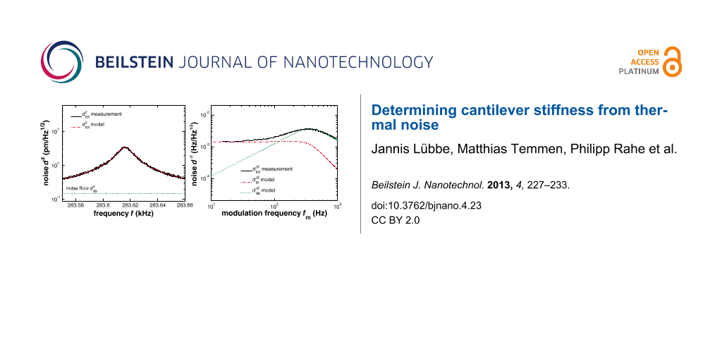
An exemplary spectrum of cantilever V 4 (see Table 1) covering the frequency region around the fundamental resonance at f0 ≈ 284 kHz is shown in Figure 1. The cantilever properties are extracted from the displacement noise spectrum by applying Equation 3. In the first step, the essentially white detection-system noise floor of the nth mode is determined by averaging the spectral density off resonance (see Figure 1a). In the second step, Equation 3 is fitted to the data with the cantilever properties f0, and as fitting parameters and as determined in the first step (see Figure 1b). Respective measurements have been performed for many cantilevers with some results compiled in Table 1, together with information on cantilever dimensions and properties measured by other techniques. Thermal noise analysis of cantilever V 4, for instance, yields = 283,616 Hz, = 28,400 and = 22 N/m. As a consistency check, we measure the cantilever response to excitation in the vicinity of the resonance, where the corresponding results for the amplitude and phase response are shown in Figure 2. A fit of the simple harmonic oscillator model to the amplitude response (Equation 3 in [12]) yields = 283,620 Hz and = 28,600 in excellent agreement with the thermal noise analysis. Generally, the fit of the thermal noise model from Equation 3 to the measured thermal excitation displacement data is excellent. In terms of experimental uncertainties, the highest precision is obtained in determining the eigenfrequency. State-of-the-art test equipment provides an accuracy of absolute frequency measurements below 1 ppm. However, practically the reproducibility is limited by thermal drift of the cantilever resonance between repeated measurements. This explains, for instance, the 4 Hz difference in the results for and for cantilever V 4 as these measurements were performed with a time difference of several hours. The reproducibility in determining the Q-factor is determined by statistical errors and can be reduced to a standard deviation of 10% for by appropriate averaging. Great care has to be taken, however, in mounting the cantilever to ensure that the measured Q-factor is the intrinsic Q-factor of the cantilever rather than an effective Q-factor caused by improper mounting of the cantilever [12]. Determining the cantilever stiffness relies on an absolute measurement of the cantilever displacement. The main limitations of precision here are the uncertainty in the calibration of the cantilever oscillation amplitude [6,17,18] and of the electronic test equipment involved. The reproducibility for the measurement of is typically 5% (standard deviation), while a comparison of to values kstat from reference measurements [16] yields an error of about 10% for the determination of stiffness from thermal noise. Note, however, that the modal stiffness k0 is related to the static stiffness k by k0 = 1.03k for a tipless cantilever while, for instance, a tip mass of 10% of the cantilever beam mass yields a relation of k0 = 1.01k instead [19].
Figure 1:
Displacement noise spectral density measured for the fundamental mode of cantilever V 4. Measurements represent the average of 50,000 spectra. (a) Measurement yielding the detection-system noise floor (dotted line). (b) Determination of , and by a fit of Equation 3 to the measured spectrum (dash-dotted line).
Figure 1:
Displacement noise spectral density measured for the fundamental mode of cantilever V 4. Measureme...
Figure 2:
(a) Measured resonance curve (solid line) of the excited cantilever V 4 with a fit (dotted line) of Equation 3 from [12] to experimental data yielding and . (b) Phase response of the excited cantilever V 4.
Figure 2:
(a) Measured resonance curve (solid line) of the excited cantilever V 4 with a fit (dotted line) of ...
In summary, the analysis of the displacement-noise spectral density around resonances of a thermally excited cantilever in a UHV environment allows the extraction of intrinsic cantilever properties with high accuracy and is specifically useful for determining modal stiffness. However, such measurements require a spectral analysis with high frequency resolution.
Stiffness from frequency shift thermal noise
To circumvent the use of a high-resolution spectrum analyser and to facilitate measurements with the test equipment that is often integrated in NC-AFM control systems, we introduce an alternative method of extracting the cantilever modal stiffness from thermal noise. To apply this method, the eigenfrequency fn and the quality factor Qn of the nth oscillation mode have to be measured from an excited resonance curve as shown in Figure 2. To determine kn, the cantilever is excited to oscillation in the nth mode at a well stabilised amplitude An. Thermal fluctuations described by the power spectral density given by Equation 1 are now superimposed to the deliberate oscillation. These fluctuations are detected by the PLL demodulator tuned to the cantilever eigenfrequency. Effectively, the PLL projects the displacement noise power spectral density in the sidebands of the mode resonance into a range of frequencies fm starting at 0 Hz. Considering the transfer function of the demodulation and the transfer function of the PLL output or loop filter Gfilter, the frequency shift noise spectral density at the PLL output can be represented as [6]
(4)
This allows us to obtain the modal stiffness from a measurement of if all other parameters are known:
(5)
Practically, the spectral analysis can be restricted to the frequency range of 10 Hz to 1 kHz. The resulting spectra are depicted in Figure 3 for different cantilevers (namely V 4 and AL 3 as described in Table 1) excited at their fundamental resonance mode at f0. The typical shape common to all such spectra has been explained in detail elsewhere [6]. The dotted and dash-dotted lines shown in Figure 3 represent the contributions from thermal noise and detection system frequency shift noise and , respectively. Here, the model curve for is not based on an independent measurement of , but determined from the measured curve assuming that the plateau indeed represents purely thermal noise. We focus on the plateau in found in the 10 to 50 Hz region. In the plateau region labelled by a representative modulation frequency , the frequency shift noise is dominated by thermal noise (fm) (dash-dotted line), while the noise contribution from the detection system (fm) (dotted line) is negligible. Within this approximation, Equation 5 can be simplified to the following expression for the modal stiffness:
(6)
Figure 3:
Frequency shift noise spectral density measured for cantilever V 4 (A0 = 16.8 nm, demodulator bandwidth B−3dB = 415 Hz) and cantilever AL 3 (A0 = 16.5 nm, demodulator bandwidth B−3dB = 258 Hz). Spectra are recorded with at least 1000 averages. Dotted lines show the contribution of the detection system noise floor; dash-dotted lines represent the contribution of the thermal noise to the total frequency shift noise . The analysis of the noise spectral density at the plateau frequency yields the cantilever stiffness according to Equation 6.
Figure 3:
Frequency shift noise spectral density measured for cantilever V 4 (A0 = 16.8 nm, demodulator band...
Prerequisite for a reliable determination of the modal stiffness is a knowledge of the cantilever properties fn and Qn and the PLL filter function Gfilter. While the former parameters can precisely be determined from an in situ cantilever excitation experiment [12], the latter function can be assumed to be 1 if the filter transfer function is reasonably well-behaved as a function of frequency and a sufficiently large PLL bandwidth is chosen [6]. Results shown in Figure 3 demonstrate that the signal quality obtained under typical experimental conditions is high enough to extract a well-defined value for () from the noise data. The modal stiffness values obtained for seven cantilevers for fundamental mode excitation according to Equation 6 are displayed in Table 1 and compared to the stiffness results obtained by using different methods for the same cantilevers. From these and further measurements (not shown here), we find an experimental uncertainty of about 20% for the modal stiffness obtained from the frequency shift noise. We attribute the decreased accuracy to noise and uncertainty in the calibration of the additional equipment involved. Note, however, that any noise source besides the thermal excitation yields a reduction in the measured modal stiffness and cannot explain values that are too high.
The determination of the effective cantilever stiffness from frequency shift noise is most interesting for cantilever excitation at higher oscillation modes where the projection of the displacement noise into the low frequency region by the PLL demodulator is especially convenient. Respective results obtained for cantilevers P 5 and AF 11 are shown in Table 2. For cantilever P 5 we obtain k1 = 154 N/m and k2 = 1330 N/m. As there is no reference for a cross-check of these values, we check for plausibility within the framework of the cantilever oscillation theory. Equation 5 given in [4] allows us to calculate the modal stiffness for a given ratio of tip mass to beam mass. Assuming the tip mass being 2% of the cantilever beam mass yields k1/k0 = 45.0 and k2/k0 = 397. These numbers fit well to the measured values for cantilever P 5 (see Table 2). The result for AF 11 can be explained by a tip mass of 5% of the cantilever beam mass.
Table 2:
Cantilever eigenfrequencies and quality factors of the nth oscillating mode for cantilevers P 5 and AF 11. The modal stiffness is obtained from the frequency shift noise spectral density through Equation 6. / is the ratio of the modal stiffness of the nth oscillation mode to the stiffness of the fundamental mode.
cantilever
n
(Hz)
(N/m)
P 5
1
436,711
44,900
154
45.3
P 5
2
1,234,277
5841
1330
391
AF 11
1
1,934,677
9000
3420
56
Conclusion
In conclusion, we introduce a method for determining the modal stiffness kn of a cantilever from frequency shift noise complemented by an independent measurement of the modal eigenfrequency and Q-factor. Our strategy yields valid results with an uncertainty of about 20%; however, the accuracy is expected to be increased by an improvement of the experimental setup. This method is particularly convenient as measurements can be performed with simple test equipment implemented in many NC-AFM control systems. Additionally, the involved spectral analysis is simple and can be performed over a bandwidth of only 1 kHz at maximum, irrespective of the cantilever eigenfrequency. We apply the thermal noise method to various cantilever types and find a good agreement of these cantilever parameters with those determined by using alternative methods. The strength of the methods presented here is that they directly yield the modal stiffness derived from a thermal measurement and do not require any modelling to relate geometric cantilever properties to oscillation properties.
Acknowledgements
The authors gratefully acknowledge experimental support from Stefan Kuhn (Johannes Gutenberg-Universität Mainz). This project has been generously supported by Nanoworld Services GmbH. M. T. gratefully appreciates support from the Hans-Mühlenhoff-Stiftung. P. R. gratefully acknowledges financial support from the Alexander von Humboldt-Foundation.
References
Nyquist, H. Phys. Rev.1928,32, 110–113.
Return to citation in text:
[1]
Johnson, J. B. Phys. Rev.1928,32, 97–109.
Return to citation in text:
[1]
Lozano, J. R.; Kiracofe, D.; Melcher, J.; Garcia, R.; Raman, A. Nanotechnology2010,21, 465502. doi:10.1088/0957-4484/21/46/465502
Return to citation in text:
[1]
[2]
In literature, two different numbering schemes for the oscillation modes are commonly used starting either with n = 0,1,2,… or n = 1,2,3,…. We use n = 0 for the fundamental oscillation mode in accordance with the nomenclature found in [6],[10],[12],[13],[15-18].
Return to citation in text:
[1]
Lübbe, J.; Temmen, M.; Rode, S.; Rahe, P.; Kühnle, A.; Reichling, M. Beilstein J. Nanotechnol.2013,4, 32–44. doi:10.3762/bjnano.4.4
Return to citation in text:
[1]
[2]
[3]
[4]
[5]
[6]
[7]
[8]
[9]
[10]
[11]
Paolino, P.; Tiribilli, B.; Bellon, L. J. Appl. Phys.2009,106, 094313. doi:10.1063/1.3245394
Return to citation in text:
[1]
Rast, S.; Wattinger, C.; Gysin, U.; Meyer, E. Nanotechnology2000,11, 169. doi:10.1088/0957-4484/11/3/306
Return to citation in text:
[1]
Hutter, J. L.; Bechhoefer, J. Rev. Sci. Instrum.1993,64, 1868–1873. doi:10.1063/1.1143970
Return to citation in text:
[1]
[2]
Cook, S. M.; Schäffer, T. E.; Chynoweth, K. M.; Wigton, M.; Simmonds, R. W.; Lang, K. M. Nanotechnology2006,17, 2135–2145. doi:10.1088/0957-4484/17/9/010
Return to citation in text:
[1]
Lantz, M. A.; Hug, H. J.; Hoffmann, R.; van Schendel, P. J. A.; Kappenberger, P.; Martin, S.; Baratoff, A.; Güntherodt, H.-J. Science2001,291, 2580–2583. doi:10.1126/science.1057824
Return to citation in text:
[1]
[2]
Kawai, S.; Glatzel, T.; Koch, S.; Baratoff, A.; Meyer, E. Phys. Rev. B2011,83, 035421. doi:10.1103/PhysRevB.83.035421
Return to citation in text:
[1]
Welker, J.; Illek, E.; Giessibl, F. J. Beilstein J. Nanotechnol.2012,3, 238–248. doi:10.3762/bjnano.3.27
Return to citation in text:
[1]
[2]
Lübbe, J.; Doering, L.; Reichling, M. Meas. Sci. Technol.2012,23, 045401. doi:10.1088/0957-0233/23/4/045401
Return to citation in text:
[1]
[2]
[3]
[4]
Giessibl, F. J. Appl. Phys. Lett.2000,76, 1470–1472. doi:10.1063/1.126067
Return to citation in text:
[1]
[2]
In literature, two different numbering schemes for the oscillation modes are commonly used starting either with n = 0,1,2,… or n = 1,2,3,…. We use n = 0 for the fundamental oscillation mode in accordance with the nomenclature found in [6],[10],[12],[13],[15-18].
Lantz, M. A.; Hug, H. J.; Hoffmann, R.; van Schendel, P. J. A.; Kappenberger, P.; Martin, S.; Baratoff, A.; Güntherodt, H.-J. Science2001,291, 2580–2583. doi:10.1126/science.1057824
Lantz, M. A.; Hug, H. J.; Hoffmann, R.; van Schendel, P. J. A.; Kappenberger, P.; Martin, S.; Baratoff, A.; Güntherodt, H.-J. Science2001,291, 2580–2583. doi:10.1126/science.1057824
Cook, S. M.; Schäffer, T. E.; Chynoweth, K. M.; Wigton, M.; Simmonds, R. W.; Lang, K. M. Nanotechnology2006,17, 2135–2145. doi:10.1088/0957-4484/17/9/010

![[Graphic 1]](/bjnano/content/inline/2190-4286-4-23-i7.svg?max-width=637&scale=1.18182) , is the superposition of contributions from all modes and can be derived within the framework of the Nyquist theory [3]. Provided the simple harmonic oscillator model is valid, i.e., the internal damping of the cantilever is small,
, is the superposition of contributions from all modes and can be derived within the framework of the Nyquist theory [3]. Provided the simple harmonic oscillator model is valid, i.e., the internal damping of the cantilever is small, ![[2190-4286-4-23-i1]](/bjnano/content/inline/2190-4286-4-23-i1.svg?max-width=590&scale=1.18182)
![[Graphic 2]](/bjnano/content/inline/2190-4286-4-23-i8.svg?max-width=637&scale=1.18182) over a limited spectral range around the resonance for a cantilever kept at a known temperature [10]. A practical implementation of this notion, focused on the determination of cantilever stiffness from thermal noise, demonstrated the validity of the approach by a critical comparison of the results against corresponding results from other methods [11].
over a limited spectral range around the resonance for a cantilever kept at a known temperature [10]. A practical implementation of this notion, focused on the determination of cantilever stiffness from thermal noise, demonstrated the validity of the approach by a critical comparison of the results against corresponding results from other methods [11].![[2190-4286-4-23-i2]](/bjnano/content/inline/2190-4286-4-23-i2.svg?max-width=590&scale=1.18182)
![[Graphic 3]](/bjnano/content/inline/2190-4286-4-23-i9.svg?max-width=637&scale=1.18182) or the corresponding power spectral density (
or the corresponding power spectral density (![[Graphic 4]](/bjnano/content/inline/2190-4286-4-23-i10.svg?max-width=637&scale=1.18182) (f))2 in a region around a specific resonance n allows the determination of the modal stiffness kn without the knowledge of any other cantilever parameters such as dimensions, shape, mass or mass distribution.
(f))2 in a region around a specific resonance n allows the determination of the modal stiffness kn without the knowledge of any other cantilever parameters such as dimensions, shape, mass or mass distribution.![[Graphic 5]](/bjnano/content/inline/2190-4286-4-23-i11.svg?max-width=637&scale=1.18182) (f) are performed by using a spectrum analyser connected to the output of the preamplifier of the position-sensitive detector of the NC-AFM instrument. The cantilever displacement is measured as a calibrated electrical signal Vz(t) and processed by the spectrum analyser [6]. For measurements of the total noise spectral density
(f) are performed by using a spectrum analyser connected to the output of the preamplifier of the position-sensitive detector of the NC-AFM instrument. The cantilever displacement is measured as a calibrated electrical signal Vz(t) and processed by the spectrum analyser [6]. For measurements of the total noise spectral density ![[Graphic 6]](/bjnano/content/inline/2190-4286-4-23-i12.svg?max-width=637&scale=1.18182) (fm) in the frequency shift signal Δf(t), the spectrum analyser is connected to the phase-locked-loop (PLL) demodulator output of the respective NC-AFM system. In all of these experiments, utmost care has to be taken to shield the NC-AFM system from mechanical and, specifically, from electric noise in spectral regions encompassing the cantilever eigenfrequencies. Otherwise measurements may be severely false due to nonthermal noise contributions. Furthermore, valid results using this methodology can only be expected for thermal noise-limited measurements performed with a system for which the PLL transfer function is known. The former condition requires the detection system noise floor
(fm) in the frequency shift signal Δf(t), the spectrum analyser is connected to the phase-locked-loop (PLL) demodulator output of the respective NC-AFM system. In all of these experiments, utmost care has to be taken to shield the NC-AFM system from mechanical and, specifically, from electric noise in spectral regions encompassing the cantilever eigenfrequencies. Otherwise measurements may be severely false due to nonthermal noise contributions. Furthermore, valid results using this methodology can only be expected for thermal noise-limited measurements performed with a system for which the PLL transfer function is known. The former condition requires the detection system noise floor ![[Graphic 7]](/bjnano/content/inline/2190-4286-4-23-i13.svg?max-width=637&scale=1.18182) to be so low that, at least over a significant fraction of the PLL demodulator bandwidth, the frequency shift noise spectral density
to be so low that, at least over a significant fraction of the PLL demodulator bandwidth, the frequency shift noise spectral density ![[Graphic 8]](/bjnano/content/inline/2190-4286-4-23-i14.svg?max-width=637&scale=1.18182) (fm) of the detection system is negligible compared to the thermal frequency-shift noise spectral density
(fm) of the detection system is negligible compared to the thermal frequency-shift noise spectral density ![[Graphic 9]](/bjnano/content/inline/2190-4286-4-23-i15.svg?max-width=637&scale=1.18182) (fm) [6].
(fm) [6].![[Graphic 10]](/bjnano/content/inline/2190-4286-4-23-i16.svg?max-width=637&scale=1.18182) (f) for the nth cantilever oscillation mode, which can be represented as [6]
(f) for the nth cantilever oscillation mode, which can be represented as [6]![[2190-4286-4-23-i3]](/bjnano/content/inline/2190-4286-4-23-i3.svg?max-width=590&scale=1.18182)
![[Graphic 16]](/bjnano/content/inline/2190-4286-4-23-i22.svg?max-width=637&scale=1.18182) (±1.5 µm) and thickness t (±0.2 µm) as provided by the manufacturer. The stiffness kdim is calculated from the cantilever dimensions, while kstat is determined by a precision measurement of the static stiffness [16]. Eigenfrequency
(±1.5 µm) and thickness t (±0.2 µm) as provided by the manufacturer. The stiffness kdim is calculated from the cantilever dimensions, while kstat is determined by a precision measurement of the static stiffness [16]. Eigenfrequency ![[Graphic 17]](/bjnano/content/inline/2190-4286-4-23-i23.svg?max-width=637&scale=1.18182) (standard deviation below 1 ppm) and quality factor
(standard deviation below 1 ppm) and quality factor ![[Graphic 18]](/bjnano/content/inline/2190-4286-4-23-i24.svg?max-width=637&scale=1.18182) (standard deviation below 1%) are obtained from a fit of the simple harmonic oscillator transfer function to the measured resonance curve of the excited cantilever [12].
(standard deviation below 1%) are obtained from a fit of the simple harmonic oscillator transfer function to the measured resonance curve of the excited cantilever [12]. ![[Graphic 19]](/bjnano/content/inline/2190-4286-4-23-i25.svg?max-width=637&scale=1.18182) and
and ![[Graphic 20]](/bjnano/content/inline/2190-4286-4-23-i26.svg?max-width=637&scale=1.18182) are the properties yielded when fitting Equation 3 to the displacement noise spectral density
are the properties yielded when fitting Equation 3 to the displacement noise spectral density ![[Graphic 21]](/bjnano/content/inline/2190-4286-4-23-i27.svg?max-width=637&scale=1.18182) of a thermally excited cantilever. The value
of a thermally excited cantilever. The value ![[Graphic 22]](/bjnano/content/inline/2190-4286-4-23-i28.svg?max-width=637&scale=1.18182) is extracted from the frequency shift noise
is extracted from the frequency shift noise ![[Graphic 23]](/bjnano/content/inline/2190-4286-4-23-i29.svg?max-width=637&scale=1.18182) from Equation 6 by using
from Equation 6 by using ![[Graphic 24]](/bjnano/content/inline/2190-4286-4-23-i30.svg?max-width=637&scale=1.18182) and
and ![[Graphic 25]](/bjnano/content/inline/2190-4286-4-23-i31.svg?max-width=637&scale=1.18182) as known parameters.
as known parameters.
![[Graphic 26]](/bjnano/content/inline/2190-4286-4-23-i32.svg?max-width=637&scale=1.18182) (µm)
(µm)
![[Graphic 27]](/bjnano/content/inline/2190-4286-4-23-i33.svg?max-width=637&scale=1.18182) (Hz)
(Hz)
![[Graphic 30]](/bjnano/content/inline/2190-4286-4-23-i36.svg?max-width=637&scale=1.18182)
![[Graphic 31]](/bjnano/content/inline/2190-4286-4-23-i37.svg?max-width=637&scale=1.18182)
![[Graphic 28]](/bjnano/content/inline/2190-4286-4-23-i34.svg?max-width=637&scale=1.18182) (N/m)
(N/m)
![[Graphic 29]](/bjnano/content/inline/2190-4286-4-23-i35.svg?max-width=637&scale=1.18182) (N/m)
(N/m)
![[Graphic 11]](/bjnano/content/inline/2190-4286-4-23-i17.svg?max-width=637&scale=1.18182) of the nth mode is determined by averaging the spectral density off resonance (see Figure 1a). In the second step, Equation 3 is fitted to the data with the cantilever properties f0,
of the nth mode is determined by averaging the spectral density off resonance (see Figure 1a). In the second step, Equation 3 is fitted to the data with the cantilever properties f0, ![[Graphic 12]](/bjnano/content/inline/2190-4286-4-23-i18.svg?max-width=637&scale=1.18182) and
and ![[Graphic 13]](/bjnano/content/inline/2190-4286-4-23-i19.svg?max-width=637&scale=1.18182) as fitting parameters and
as fitting parameters and ![[Graphic 14]](/bjnano/content/inline/2190-4286-4-23-i20.svg?max-width=637&scale=1.18182) as determined in the first step (see Figure 1b). Respective measurements have been performed for many cantilevers with some results compiled in Table 1, together with information on cantilever dimensions and properties measured by other techniques. Thermal noise analysis of cantilever V 4, for instance, yields
as determined in the first step (see Figure 1b). Respective measurements have been performed for many cantilevers with some results compiled in Table 1, together with information on cantilever dimensions and properties measured by other techniques. Thermal noise analysis of cantilever V 4, for instance, yields ![[Graphic 15]](/bjnano/content/inline/2190-4286-4-23-i21.svg?max-width=637&scale=1.18182) = 283,616 Hz,
= 283,616 Hz, ![[Graphic 32]](/bjnano/content/inline/2190-4286-4-23-i38.svg?max-width=637&scale=1.18182) = 283,620 Hz and
= 283,620 Hz and ![[Graphic 33]](/bjnano/content/inline/2190-4286-4-23-i39.svg?max-width=637&scale=1.18182) = 28,600 in excellent agreement with the thermal noise analysis. Generally, the fit of the thermal noise model from Equation 3 to the measured thermal excitation displacement data is excellent. In terms of experimental uncertainties, the highest precision is obtained in determining the eigenfrequency. State-of-the-art test equipment provides an accuracy of absolute frequency measurements below 1 ppm. However, practically the reproducibility is limited by thermal drift of the cantilever resonance between repeated measurements. This explains, for instance, the 4 Hz difference in the results for
= 28,600 in excellent agreement with the thermal noise analysis. Generally, the fit of the thermal noise model from Equation 3 to the measured thermal excitation displacement data is excellent. In terms of experimental uncertainties, the highest precision is obtained in determining the eigenfrequency. State-of-the-art test equipment provides an accuracy of absolute frequency measurements below 1 ppm. However, practically the reproducibility is limited by thermal drift of the cantilever resonance between repeated measurements. This explains, for instance, the 4 Hz difference in the results for ![[2190-4286-4-23-1]](/bjnano/content/figures/2190-4286-4-23-1.svg?scale=1.6&max-width=1024&background=FFFFFF)
![[Graphic 34]](/bjnano/content/inline/2190-4286-4-23-i40.svg?max-width=637&scale=1.18182) measured for the fundamental mode of cantilever V 4. Measurements represent the average of 50,000 spectra. (a) Measurement yielding the detection-system noise floor
measured for the fundamental mode of cantilever V 4. Measurements represent the average of 50,000 spectra. (a) Measurement yielding the detection-system noise floor ![[Graphic 35]](/bjnano/content/inline/2190-4286-4-23-i41.svg?max-width=637&scale=1.18182) (dotted line). (b) Determination of
(dotted line). (b) Determination of ![[Graphic 36]](/bjnano/content/inline/2190-4286-4-23-i42.svg?max-width=637&scale=1.18182) ,
, ![[2190-4286-4-23-2]](/bjnano/content/figures/2190-4286-4-23-2.svg?scale=1.6&max-width=1024&background=FFFFFF)
![[2190-4286-4-23-i4]](/bjnano/content/inline/2190-4286-4-23-i4.svg?max-width=590&scale=1.18182)
![[Graphic 37]](/bjnano/content/inline/2190-4286-4-23-i43.svg?max-width=637&scale=1.18182) if all other parameters are known:
if all other parameters are known:![[2190-4286-4-23-i5]](/bjnano/content/inline/2190-4286-4-23-i5.svg?max-width=590&scale=1.18182)
![[Graphic 38]](/bjnano/content/inline/2190-4286-4-23-i44.svg?max-width=637&scale=1.18182) and
and ![[Graphic 39]](/bjnano/content/inline/2190-4286-4-23-i45.svg?max-width=637&scale=1.18182) , respectively. Here, the model curve for
, respectively. Here, the model curve for ![[Graphic 40]](/bjnano/content/inline/2190-4286-4-23-i46.svg?max-width=637&scale=1.18182) , but determined from the measured
, but determined from the measured ![[Graphic 41]](/bjnano/content/inline/2190-4286-4-23-i47.svg?max-width=637&scale=1.18182) , the frequency shift noise is dominated by thermal noise
, the frequency shift noise is dominated by thermal noise ![[2190-4286-4-23-i6]](/bjnano/content/inline/2190-4286-4-23-i6.svg?max-width=590&scale=1.18182)
![[2190-4286-4-23-3]](/bjnano/content/figures/2190-4286-4-23-3.svg?scale=1.6&max-width=1024&background=FFFFFF)
![[Graphic 42]](/bjnano/content/inline/2190-4286-4-23-i48.svg?max-width=637&scale=1.18182) of the detection system noise floor; dash-dotted lines represent the contribution
of the detection system noise floor; dash-dotted lines represent the contribution ![[Graphic 43]](/bjnano/content/inline/2190-4286-4-23-i49.svg?max-width=637&scale=1.18182) of the thermal noise to the total frequency shift noise
of the thermal noise to the total frequency shift noise ![[Graphic 44]](/bjnano/content/inline/2190-4286-4-23-i50.svg?max-width=637&scale=1.18182) yields the cantilever stiffness
yields the cantilever stiffness ![[Graphic 45]](/bjnano/content/inline/2190-4286-4-23-i51.svg?max-width=637&scale=1.18182) according to Equation 6.
according to Equation 6.
![[Graphic 46]](/bjnano/content/inline/2190-4286-4-23-i52.svg?max-width=637&scale=1.18182) obtained for seven cantilevers for fundamental mode excitation according to Equation 6 are displayed in Table 1 and compared to the stiffness results obtained by using different methods for the same cantilevers. From these and further measurements (not shown here), we find an experimental uncertainty of about 20% for the modal stiffness obtained from the frequency shift noise. We attribute the decreased accuracy to noise and uncertainty in the calibration of the additional equipment involved. Note, however, that any noise source besides the thermal excitation yields a reduction in the measured modal stiffness and cannot explain values that are too high.
obtained for seven cantilevers for fundamental mode excitation according to Equation 6 are displayed in Table 1 and compared to the stiffness results obtained by using different methods for the same cantilevers. From these and further measurements (not shown here), we find an experimental uncertainty of about 20% for the modal stiffness obtained from the frequency shift noise. We attribute the decreased accuracy to noise and uncertainty in the calibration of the additional equipment involved. Note, however, that any noise source besides the thermal excitation yields a reduction in the measured modal stiffness and cannot explain values that are too high.![[Graphic 47]](/bjnano/content/inline/2190-4286-4-23-i53.svg?max-width=637&scale=1.18182) and quality factors
and quality factors ![[Graphic 48]](/bjnano/content/inline/2190-4286-4-23-i54.svg?max-width=637&scale=1.18182) of the nth oscillating mode for cantilevers P 5 and AF 11. The modal stiffness
of the nth oscillating mode for cantilevers P 5 and AF 11. The modal stiffness ![[Graphic 49]](/bjnano/content/inline/2190-4286-4-23-i55.svg?max-width=637&scale=1.18182) through Equation 6.
through Equation 6. ![[Graphic 50]](/bjnano/content/inline/2190-4286-4-23-i56.svg?max-width=637&scale=1.18182) (Hz)
(Hz)
![[Graphic 51]](/bjnano/content/inline/2190-4286-4-23-i57.svg?max-width=637&scale=1.18182)
![[Graphic 52]](/bjnano/content/inline/2190-4286-4-23-i58.svg?max-width=637&scale=1.18182) (N/m)
(N/m)
![[Graphic 53]](/bjnano/content/inline/2190-4286-4-23-i59.svg?max-width=637&scale=1.18182)