Abstract
The diode effect in superconducting materials has been actively investigated in recent years. Plenty of different devices have been proposed as a platform to observe the superconducting diode effect. In this work, we discuss the possibility of a highly efficient superconducting diode design with controllable polarity. We propose a mesoscopic device that consists of two separated superconducting islands with proximity-induced ferromagnetism deposited on top of a three-dimensional topological insulator. Using the quasiclassical formalism of the Usadel equations, we demonstrate that the sign of the diode efficiency can be controlled by magnetization tuning of a single superconducting island. Moreover, we show that the diode efficiency can be substantially increased in such a device. We argue that the dramatic increase of the diode efficiency is due to competing contributions of the two superconducting islands to the supercurrent with single helical bands linked through the topological insulator surface.
Introduction
Superconducting nonreciprocal phenomena have been attracting a lot of attention over the last several years [1]. Particularly, the diode effect in superconducting systems has been widely discussed due to its interesting underlying physics and potential application in nondissipative superconducting electronics [2-4]. So far, the superconducting diode effect has been reported in many different systems, including Josephson junctions [5-11], junction-free devices [12-17], superconducting microbridges [18,19], and other systems [20,21]. There have been numerous theoretical propositions demonstrating the possibility of the superconducting diode effect such as bulk superconducting materials [22-34], proximity-effect hybrid structures [35-45], Josephson structures [46-65], nanotubes [66], confined systems [67], asymmetric SQUIDs [68-70], and superconducting systems with nonuniform magnetization [71]. The diode effect might be useful not only from an application point of view, but it may be also employed as a way to detect the spin–orbital coupling (SOC) type of the material [72].
Typically, such devices require three ingredients for achieving the nonreciprocity of the critical current, including lack of inversion and time-reversal symmetries and the presence of the superconducting order parameter [1]. However, it should be emphasized that the lack of inversion symmetry is the implication of the gyrotropy in the structure of the material that supports nonreciprocal transport [39]. On the microscopic level, the lack of inversion symmetry is expressed by the SOC term. In this regard, systems based on topological insulators (TIs) are interesting since they offer strongest SOC rendering linear spin-polarized dispersion for the surface states [73].
The diode effect in TI-based structures has been reported in Josephson junctions, as well as in hybrid structures. In practice, when producing mesoscopic diode devices, it is reasonable to expect some presence of nonmagnetic impurities in the structures. However, it has been shown previously that the diode efficiency is expected to be low in diffusive TI-based systems [37,50]. Another disadvantage of the TI diffusive diodes is their limited tunability. In these devices, the polarity of the diode cannot be changed without reversing the Zeeman field, although in long ballistic S/TI/S (S denotes a superconductor) Josephson junctions such a situation is possible [52].
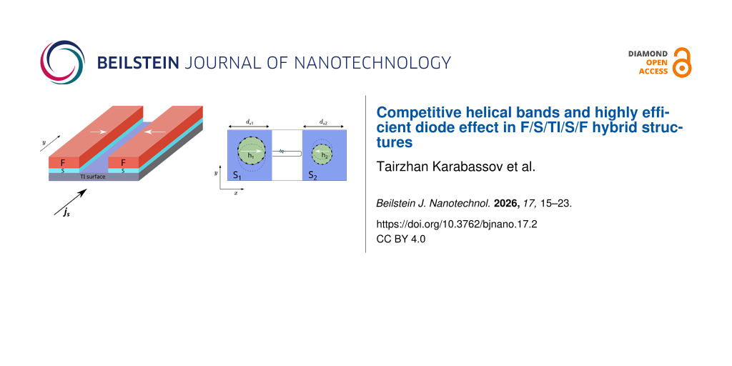
In the present work, we propose a superconducting diode based on two superconducting regions with a proximity-induced in-plane exchange field on top of the TI. The Fermi contour of the TI surface states is usually represented by the Dirac spectrum, that is, a single helical band, which is characterized by the strongest spin-momentum locking effect. Here, we consider the F/S/TI/S/F (F denotes ferromagnetic layer) hybrid structure depicted in Figure 1. We argue that such a hybrid structure can behave as a system with two helical bands as, for example, noncentrosymmetric superconductors [26,74]. However, the two helical bands in the structure under consideration are coupled not in the momentum space but in the real space by the TI surface. The coupling between the two islands can be controlled, for example, by the width of the non-superconducting TI part. When considering the diode effect, the proposed layout can substantially increase the diode efficiency, provided the ferromagnetic exchange fields of the two F/S regions are oriented in opposite directions. Misalignment of the exchange fields leads to the competition of the two separate helical bands in the superconducting regions in their contribution to the critical current nonreciprocity (Figure 1).
![[2190-4286-17-2-1]](/bjnano/content/figures/2190-4286-17-2-1.png?scale=2.0&max-width=1024&background=FFFFFF)
Figure 1: Geometry of the controllable diode under consideration, which consists of two superconducting islands with the proximity-induced in-plane exchange field deposited on top of the topological insulator. Schematic representation of the Fermi contours of the two superconducting regions with the exchange fields oriented in the opposite directions. S1 and S2 are linked through the TI surface.
Figure 1: Geometry of the controllable diode under consideration, which consists of two superconducting islan...
Quasiclassical Theory
The F/S/TI/S/F hybrid structure can be described by the following effective low-energy Hamiltonian in the particle–hole and spin space:
![[2190-4286-17-2-i1]](/bjnano/content/inline/2190-4286-17-2-i1.svg?max-width=590&scale=1.18182)
where α is the Fermi velocity, μ is the chemical potential, and V is the impurity potential of a Gaussian form, which is used for further quasiclassical approximation in the dirty limit. h = (hx, 0, 0) is the exchange field due to the adjacent ferromagnetic material. The matrices τ and σ are 2 × 2 Pauli matrices in the particle–hole and spin spaces, respectively. The superconducting pair potential matrix ![[Graphic 1]](/bjnano/content/inline/2190-4286-17-2-i16.svg?max-width=637&scale=1.18182) is defined as
is defined as ![[Graphic 2]](/bjnano/content/inline/2190-4286-17-2-i17.svg?max-width=637&scale=1.18182) , where the transformation matrix is
, where the transformation matrix is ![[Graphic 3]](/bjnano/content/inline/2190-4286-17-2-i18.svg?max-width=637&scale=1.18182) . The finite center of mass momentum q takes into account the helical state. The pair potential Δ(x) is a real function defined as follows:
. The finite center of mass momentum q takes into account the helical state. The pair potential Δ(x) is a real function defined as follows:
![[2190-4286-17-2-i2]](/bjnano/content/inline/2190-4286-17-2-i2.svg?max-width=590&scale=1.18182)
Here, Δ1 and Δ2 are calculated self-consistently and correspond to the superconducting regions S1 and S2, respectively (Figure 1). Finally, L is the width of the bare TI surface (normal N part) and ds1(ds2) is the width of S1 (S2) region. It is important to emphasize that, although the geometry of the considered device corresponds to a Josephson junction, in this work we consider zero macroscopic phase difference between regions S1 and S2, so that the Josephson supercurrent due to the phase shift is absent. The anomalous ground state phase shift ϕ0 is also absent since we assume the exchange field component hy = 0. In contrast, the hx component is considered to be finite in the system and defined as follows:
![[2190-4286-17-2-i3]](/bjnano/content/inline/2190-4286-17-2-i3.svg?max-width=590&scale=1.18182)
As we stated above, we assume the phase gradient q to be the same in the whole system. Obviously, this is not the case if L ≫ ξ because, in this case, the Josephson coupling between the S1 and S2 leads is absent, and they do not “feel” each other. In each lead, a distinct phase gradient q1,2 = −2hi/α is established to satisfy the zero spontaneous current condition required for the helical ground state [37,75,76]. If the superconducting leads get closer to each other, Josephson coupling between them develops gradually, and Josephson currents between the leads appear. Consequently, the distribution of the superconducting phase becomes a complex two-dimensional function of spatial coordinates. Thus, a general solution of the problem requires a consideration of the two-dimensional distribution of the order parameter phase; but here we restrict ourselves to the case ![[Graphic 4]](/bjnano/content/inline/2190-4286-17-2-i19.svg?max-width=637&scale=1.18182) and the regime of relatively strong Josephson coupling between the leads S1 and S2. The second condition means that
and the regime of relatively strong Josephson coupling between the leads S1 and S2. The second condition means that ![[Graphic 5]](/bjnano/content/inline/2190-4286-17-2-i20.svg?max-width=637&scale=1.18182) , and the transparency of the interfaces between the superconducting leads and the TI layer is rather high. In this case, it is energetically favorable to have the same phase gradient along the whole S1/TI/S2 Josephson junction and the key results are obtained within this regime.
, and the transparency of the interfaces between the superconducting leads and the TI layer is rather high. In this case, it is energetically favorable to have the same phase gradient along the whole S1/TI/S2 Josephson junction and the key results are obtained within this regime.
In practice, one possible implementation of the hybrid structure includes a thin layer of Nb on the surface of Bi2Se3 with FeMn- or CuNi-based ferromagnets deposited on top of the superconductors. Despite the challenges, it is still possible to implement heterostructures with opposite magnetization directions as in, for example, F/S/F spin valves [77]. Another possibility is more modern and is based on van der Waals structures comprised of transition-metal dichalcogenide materials such as superconducting NbSe2 and magnetic VSe2 on top of Bi2Se3 [78].
We solve the stated problem for the Hamiltonian in Equation 1 within the microscopic approach based on the quasiclassical Green’s functions in the diffusive limit, that is, when the coherence length ξ is much larger than the electron mean free path l. Such model can be described by the Usadel equations [79-81]
![[2190-4286-17-2-i4]](/bjnano/content/inline/2190-4286-17-2-i4.svg?max-width=590&scale=1.18182)
Here D is the diffusion constant, and τz is the Pauli matrix in the particle–hole space. In the general case, the operator ![[Graphic 6]](/bjnano/content/inline/2190-4286-17-2-i21.svg?max-width=637&scale=1.18182) . The Green’s function matrix is also transformed as
. The Green’s function matrix is also transformed as ![[Graphic 7]](/bjnano/content/inline/2190-4286-17-2-i22.svg?max-width=637&scale=1.18182) .
.
To facilitate the solution procedures of the nonlinear Usadel equations, we employ θ parametrization of the Green’s functions [82]:
![[2190-4286-17-2-i5]](/bjnano/content/inline/2190-4286-17-2-i5.svg?max-width=590&scale=1.18182)
Substituting the above matrix into the Usadel equation (Equation 4), we obtain in the superconducting S parts |x| > L/2:
![[2190-4286-17-2-i6]](/bjnano/content/inline/2190-4286-17-2-i6.svg?max-width=590&scale=1.18182)
where the indices i = 1, 2 refer to the superconducting parts S1 and S2, respectively, qi = q + 2hi/α, and in the normal N part −L/2 < x < L/2:
![[2190-4286-17-2-i7]](/bjnano/content/inline/2190-4286-17-2-i7.svg?max-width=590&scale=1.18182)
where θs(N) means the value of θ is the S(N) of the TI surface, respectively. We introduced the characteristic length ![[Graphic 8]](/bjnano/content/inline/2190-4286-17-2-i23.svg?max-width=637&scale=1.18182) , where Ds(N) is the diffusion constant in S(N) part and Tcs is the transition temperature of the bare S region. The self-consistency equations for the pair potentials read
, where Ds(N) is the diffusion constant in S(N) part and Tcs is the transition temperature of the bare S region. The self-consistency equations for the pair potentials read
![[2190-4286-17-2-i8]](/bjnano/content/inline/2190-4286-17-2-i8.svg?max-width=590&scale=1.18182)
where the summation is performed up to the Debye frequency ωD. Finally, we supplement the above equations with two pairs of the boundary conditions (two for each S/N interface) of the following type:
![[2190-4286-17-2-i9]](/bjnano/content/inline/2190-4286-17-2-i9.svg?max-width=590&scale=1.18182)
![[2190-4286-17-2-i10]](/bjnano/content/inline/2190-4286-17-2-i10.svg?max-width=590&scale=1.18182)
Here, γB = RBσl/ξl, γ = ξrσl/ξlσr where σl(r) is the conductivity of the material on the left (right) side of the interface. The parameter γ controls the slope of the Green’s functions at the interface, whereas γB controls the mismatch between the functions at the interface. While for identical materials γ = 1, in general, this parameter may have arbitrary values. γB is the parameter that determines the transparency of the S/F interface [83-85].
The final problem comprises several equations, namely, the Usadel equations in the superconducting (S) and normal (N) parts (Equation 6 and Equation 7), two self-consistency equations (Equation 8) in each superconducting region S1 and S2, and the boundary conditions at the S1/N, N/S2 interfaces and at the free edges of the superconductors. These equations are solved simultaneously for a given phase gradient q. Using the finite difference method, the equations are discretized on a one-dimensional grid, resulting in a system of nonlinear equations that is solved by the Newton–Raphson method. We then compute the total supercurrent through the hybrid structure as a function of q, from which the supercurrent and critical current of the system are determined.
The supercurrent in the diffusive limit can be found from the expression
![[2190-4286-17-2-i11]](/bjnano/content/inline/2190-4286-17-2-i11.svg?max-width=590&scale=1.18182)
Performing the unitary transformation U, the current density transforms as follows:
![[2190-4286-17-2-i12]](/bjnano/content/inline/2190-4286-17-2-i12.svg?max-width=590&scale=1.18182)
![[2190-4286-17-2-i13]](/bjnano/content/inline/2190-4286-17-2-i13.svg?max-width=590&scale=1.18182)
The total supercurrent flowing through the system along the y-direction can be calculated by integrating the current density of the total width of the F/S/TI/S/F structure:
![[2190-4286-17-2-i14]](/bjnano/content/inline/2190-4286-17-2-i14.svg?max-width=590&scale=1.18182)
where Is1, Is2, and IN are the total supercurrents integrated along the x-direction in S1, S2 and N regions, respectively.
Results and Discussion
We fix the following system parameters throughout the discussion of the results: ds1 = ds2 = 1.2ξ, γ1 = γ2 = 0.5, T = 0.1Tcs. We start with the analysis of the I(q) relations when the exchange fields H1 and H2 are the same in both superconducting regions. In Figure 2a, we observe a characteristic behavior of the supercurrent with I(q0) = 0, where q0 ≠ 0 is the ground-state Cooper pair momentum, which reflects the helical nature of the superconducting ground state. We can also notice some nonreciprocity of the supercurrent, that is, ![[Graphic 9]](/bjnano/content/inline/2190-4286-17-2-i24.svg?max-width=637&scale=1.18182) , which is a consequence of the helical state. As we will see below, the diode efficiency is quite low and, in this case, does not exceed several percent. In the absence of any exchange field, the supercurrent is I(q = 0) = 0, which means that the ground state is a conventional state with zero Cooper pair momentum. To get more insight, we plot the supercurrent density Jy in Figure 2b. Hence, in the situation when H1 and H2 are perfectly aligned, we expect well-known behavior of the total supercurrent.
, which is a consequence of the helical state. As we will see below, the diode efficiency is quite low and, in this case, does not exceed several percent. In the absence of any exchange field, the supercurrent is I(q = 0) = 0, which means that the ground state is a conventional state with zero Cooper pair momentum. To get more insight, we plot the supercurrent density Jy in Figure 2b. Hence, in the situation when H1 and H2 are perfectly aligned, we expect well-known behavior of the total supercurrent.
![[2190-4286-17-2-2]](/bjnano/content/figures/2190-4286-17-2-2.png?scale=2.0&max-width=1024&background=FFFFFF)
Figure 2: Supercurrent I as a function of q at h1 = h2 = 0.25 (a) and at h1 = −0.1, h2 = 0.25 (b). The lower panels illustrate the current density distributions at different q corresponding to the upper panels for L = ξ.
Figure 2: Supercurrent I as a function of q at h1 = h2 = 0.25 (a) and at h1 = −0.1, h2 = 0.25 (b). The lower ...
Now, we discuss the case when the exchange fields H1 and H2 are oriented in opposite directions (Figure 2b). When the distance between S1 and S2 is large (L = 4ξ), the superconducting regions are well separated and act almost independently with distinct critical supercurrents ![[Graphic 10]](/bjnano/content/inline/2190-4286-17-2-i25.svg?max-width=637&scale=1.18182) and
and ![[Graphic 11]](/bjnano/content/inline/2190-4286-17-2-i26.svg?max-width=637&scale=1.18182) corresponding to S1 and S2, respectively. This circumstance can be clearly seen from I(q) dependence for L = 4ξ; in this sense, the distance L can be imagined as a coupling strength between S1 and S2. The behavior of I(q) dramatically changes when L becomes smaller. The regions of the I(q) curve that previously could be easily assigned to each superconducting island start to “overlap”, reflecting stronger coupling between S1 and S2. As a result, we can achieve a situation in which the critical current of the hybrid structure in one direction is substantially renormalized. For instance, we can observe that
corresponding to S1 and S2, respectively. This circumstance can be clearly seen from I(q) dependence for L = 4ξ; in this sense, the distance L can be imagined as a coupling strength between S1 and S2. The behavior of I(q) dramatically changes when L becomes smaller. The regions of the I(q) curve that previously could be easily assigned to each superconducting island start to “overlap”, reflecting stronger coupling between S1 and S2. As a result, we can achieve a situation in which the critical current of the hybrid structure in one direction is substantially renormalized. For instance, we can observe that ![[Graphic 12]](/bjnano/content/inline/2190-4286-17-2-i27.svg?max-width=637&scale=1.18182) is defined rather by the left maximum of I(q) at L = ξ, while
is defined rather by the left maximum of I(q) at L = ξ, while ![[Graphic 13]](/bjnano/content/inline/2190-4286-17-2-i28.svg?max-width=637&scale=1.18182) remains approximately at the same value. Stronger coupling between the superconducting regions leads to a more complicated supercurrent density distribution across the hybrid structure (see Figure 2d). Obtaining such nontrivial behavior of I(q) is the key idea behind achieving a larger diode efficiency η. It should be emphasized that a similar behavior is expected in Rashba superconductors, where the Fermi surface is represented by the two helical bands with the opposite helicities [24-26]. Here, we clearly consider a single-helical-band Fermi surface. However, we can have S1 and S2 with the opposite h1 and h2 in our system as illustrated in Figure 1, which may be thought of as an effective two-helical-bands system.
remains approximately at the same value. Stronger coupling between the superconducting regions leads to a more complicated supercurrent density distribution across the hybrid structure (see Figure 2d). Obtaining such nontrivial behavior of I(q) is the key idea behind achieving a larger diode efficiency η. It should be emphasized that a similar behavior is expected in Rashba superconductors, where the Fermi surface is represented by the two helical bands with the opposite helicities [24-26]. Here, we clearly consider a single-helical-band Fermi surface. However, we can have S1 and S2 with the opposite h1 and h2 in our system as illustrated in Figure 1, which may be thought of as an effective two-helical-bands system.
The diode efficiency can be defined in a standard way, as
![[2190-4286-17-2-i15]](/bjnano/content/inline/2190-4286-17-2-i15.svg?max-width=590&scale=1.18182)
In Figure 3, the diode efficiency along with the critical currents is demonstrated as a function of H1, while H2 is fixed at H2 = 0.25. We observe several characteristic features of η behavior. First, the diode efficiency is quite low at large positive values of H1, remaining under 5% at H1 = 0.1. This is anticipated behavior of the diodes with single helical band in the diffusive limit [37,50,86]. As H1 decreases, the diode efficiency rises to a certain value, and then η changes its sign rapidly reaching the maximum value. At the point when the diode changes its polarity, there is a transition from S1 to S2 in their contribution to the critical currents. We assume that in the vicinity of η = 0, the superconducting regions S1 and S2 strongly compete with each other since, individually, they have opposite efficiencies because H1 and H2 are of the opposite signs. We might say that, at a certain value of H1, the critical currents ![[Graphic 14]](/bjnano/content/inline/2190-4286-17-2-i29.svg?max-width=637&scale=1.18182) and
and ![[Graphic 15]](/bjnano/content/inline/2190-4286-17-2-i30.svg?max-width=637&scale=1.18182) of the total system are predominantly determined by S1 and S2, that is, the supercurrent mostly passes through one of the superconducting regions in the opposite directions. To better demonstrate this point, we plot the supercurrent density distribution (Figure 4) for values of q that correspond to the critical current momenta at H1 = −0.1, H2 = 0.25, and L = ξ. It can be seen that a larger proportion of the current density is concentrated at the corresponding superconducting region; at qξ = 0.35, Jy is significantly larger at S1, while at qξ = −0.58, it is mainly at S2. Another important observation from Figure 3 is that the sign change of the diode efficiency occurs at lower values of the critical currents. This means that higher diode efficiencies due to the competition of S1 and S2 take place in a substantially suppressed superconducting state. Finally, we can see how the interface transparency affects η. Higher transparency can increase the efficiency up to 40%, however at smaller critical currents.
of the total system are predominantly determined by S1 and S2, that is, the supercurrent mostly passes through one of the superconducting regions in the opposite directions. To better demonstrate this point, we plot the supercurrent density distribution (Figure 4) for values of q that correspond to the critical current momenta at H1 = −0.1, H2 = 0.25, and L = ξ. It can be seen that a larger proportion of the current density is concentrated at the corresponding superconducting region; at qξ = 0.35, Jy is significantly larger at S1, while at qξ = −0.58, it is mainly at S2. Another important observation from Figure 3 is that the sign change of the diode efficiency occurs at lower values of the critical currents. This means that higher diode efficiencies due to the competition of S1 and S2 take place in a substantially suppressed superconducting state. Finally, we can see how the interface transparency affects η. Higher transparency can increase the efficiency up to 40%, however at smaller critical currents.
![[2190-4286-17-2-3]](/bjnano/content/figures/2190-4286-17-2-3.png?scale=2.0&max-width=1024&background=FFFFFF)
Figure 3:
Critical supercurrents ![[Graphic 16]](/bjnano/content/inline/2190-4286-17-2-i31.svg?max-width=637&scale=1.18182) and
and ![[Graphic 17]](/bjnano/content/inline/2190-4286-17-2-i32.svg?max-width=637&scale=1.18182) (right vertical scale) and diode efficiency η (left vertical scale) as functions of H1 for L = ξ. Left and right plots correspond to γB1 = γB2 = 0.4 and γB1 = γB2 = 0.2, respectively. The critical currents’ scale is in units of 2e/πkTcσnξ.
(right vertical scale) and diode efficiency η (left vertical scale) as functions of H1 for L = ξ. Left and right plots correspond to γB1 = γB2 = 0.4 and γB1 = γB2 = 0.2, respectively. The critical currents’ scale is in units of 2e/πkTcσnξ.
Figure 3:
Critical supercurrents and (right vertical scale) and diode efficiency η (left vertical scale) as...
![[2190-4286-17-2-4]](/bjnano/content/figures/2190-4286-17-2-4.png?scale=2.0&max-width=1024&background=FFFFFF)
Figure 4: Supercurrent density Jy at qξ = −0.58 (black line) and qξ = 0.35 (red line) calculated at L = ξ. All other parameters are the same as in Figure 3.
Figure 4: Supercurrent density Jy at qξ = −0.58 (black line) and qξ = 0.35 (red line) calculated at L = ξ. Al...
The interface transparency γB is an important parameter of the system, which, in principle, can be used as a tuning parameter in the experiment. Control of this parameter may be achieved by applying the gating voltage at the interface. We provide more detailed analysis of the interface transparency impact on the diode effect in Figure 5. We notice that the highest efficiency is achieved at smaller γB = 0.2 for L = ξ. However, this is not the general trend as we see from the plots. For instance, the highest η is realized at γB = 0.5 for L = 4ξ. Hence, there exists an optimal value of the interface transparency for the highest efficiency. It is also important to emphasize that the exchange field H1 at which the “major” sign change of η occurs shifts towards larger values as γB decreases. This means that the polarity of the diode can be altered via the control of the interface transparency, which cannot be achieved in a diffusive single-helical-band superconducting diode [37]. Finally, we observe repeated sign-changing behavior of the quality factor in Figure 5. This may reflect the competitive nature of the S1 and S2 behavior in the nonreciprocal supercurrent.
![[2190-4286-17-2-5]](/bjnano/content/figures/2190-4286-17-2-5.png?scale=2.0&max-width=1024&background=FFFFFF)
Figure 5: Superconducting diode efficiency η calculated at different interface transparencies γB. Plot (a) corresponds to γB1 = γB2 = 0.5, (b) γB1 = γB2 = 0.4, (c) γB1 = γB2 = 0.3, and (d) γB1 = γB2 = 0.2.
Figure 5: Superconducting diode efficiency η calculated at different interface transparencies γB. Plot (a) co...
Conclusion
We have examined the superconducting diode effect in a F/S/TI/S/F hybrid structure. It has been shown that, under the condition that the exchange fields of the ferromagnetic regions are opposite, the diode efficiency can be dramatically increased. Such improvement can be explained in terms of the competitive behavior of the superconducting regions with single helical bands. The obtained results can be useful for achieving highly efficient superconducting diodes in the absence of an external magnetic field. Moreover, the sign of the diode efficiency can be changed as a function of the interface transparency.
As a direction for further studies, one could investigate the Josephson diode effect in the hybrid structure considered in this paper. In this case, the nonreciprocity is achieved in the Josephson critical current.
Funding
The analytical calculations were supported by MIPT via the project FSMG-2023-0014. The numerical calculations were supported by the megagrant of the Ministry of Science and Higher Education of Russian Federation No. 075-15-2024-632. T. K acknowledge the support from the Foundation for the Advancement of Theoretical Physics and Mathematics “BASIS” via the project number 25-1-4-21-1. T. K. and P. M. acknowledge the support of the HSE University Basic Research Program that was used to develop the model.
Data Availability Statement
Data generated and analyzed during this study is available from the corresponding author upon reasonable request.
References
-
Nadeem, M.; Fuhrer, M. S.; Wang, X. Nat. Rev. Phys. 2023, 5, 558–577. doi:10.1038/s42254-023-00632-w
Return to citation in text: [1] [2] -
Soloviev, I. I.; Klenov, N. V.; Bakurskiy, S. V.; Kupriyanov, M. Y.; Gudkov, A. L.; Sidorenko, A. S. Beilstein J. Nanotechnol. 2017, 8, 2689–2710. doi:10.3762/bjnano.8.269
Return to citation in text: [1] -
Linder, J.; Robinson, J. W. A. Nat. Phys. 2015, 11, 307–315. doi:10.1038/nphys3242
Return to citation in text: [1] -
Eschrig, M. Rep. Prog. Phys. 2015, 78, 104501. doi:10.1088/0034-4885/78/10/104501
Return to citation in text: [1] -
Golod, T.; Krasnov, V. M. Nat. Commun. 2022, 13, 3658. doi:10.1038/s41467-022-31256-w
Return to citation in text: [1] -
Wu, H.; Wang, Y.; Xu, Y.; Sivakumar, P. K.; Pasco, C.; Filippozzi, U.; Parkin, S. S. P.; Zeng, Y.-J.; McQueen, T.; Ali, M. N. Nature 2022, 604, 653–656. doi:10.1038/s41586-022-04504-8
Return to citation in text: [1] -
Baumgartner, C.; Fuchs, L.; Costa, A.; Reinhardt, S.; Gronin, S.; Gardner, G. C.; Lindemann, T.; Manfra, M. J.; Faria Junior, P. E.; Kochan, D.; Fabian, J.; Paradiso, N.; Strunk, C. Nat. Nanotechnol. 2022, 17, 39–44. doi:10.1038/s41565-021-01009-9
Return to citation in text: [1] -
Pal, B.; Chakraborty, A.; Sivakumar, P. K.; Davydova, M.; Gopi, A. K.; Pandeya, A. K.; Krieger, J. A.; Zhang, Y.; Date, M.; Ju, S.; Yuan, N.; Schröter, N. B. M.; Fu, L.; Parkin, S. S. P. Nat. Phys. 2022, 18, 1228–1233. doi:10.1038/s41567-022-01699-5
Return to citation in text: [1] -
Chen, C.-Z.; He, J. J.; Ali, M. N.; Lee, G.-H.; Fong, K. C.; Law, K. T. Phys. Rev. B 2018, 98, 075430. doi:10.1103/physrevb.98.075430
Return to citation in text: [1] -
Trahms, M.; Melischek, L.; Steiner, J. F.; Mahendru, B.; Tamir, I.; Bogdanoff, N.; Peters, O.; Reecht, G.; Winkelmann, C. B.; von Oppen, F.; Franke, K. J. Nature 2023, 615, 628–633. doi:10.1038/s41586-023-05743-z
Return to citation in text: [1] -
Yu, W.; Cuozzo, J. J.; Sapkota, K.; Rossi, E.; Rademacher, D. X.; Nenoff, T. M.; Pan, W. Phys. Rev. B 2024, 110, 104510. doi:10.1103/physrevb.110.104510
Return to citation in text: [1] -
Ando, F.; Miyasaka, Y.; Li, T.; Ishizuka, J.; Arakawa, T.; Shiota, Y.; Moriyama, T.; Yanase, Y.; Ono, T. Nature 2020, 584, 373–376. doi:10.1038/s41586-020-2590-4
Return to citation in text: [1] -
Narita, H.; Ishizuka, J.; Kawarazaki, R.; Kan, D.; Shiota, Y.; Moriyama, T.; Shimakawa, Y.; Ognev, A. V.; Samardak, A. S.; Yanase, Y.; Ono, T. Nat. Nanotechnol. 2022, 17, 823–828. doi:10.1038/s41565-022-01159-4
Return to citation in text: [1] -
Itahashi, Y.; Ideue, T.; Saito, Y.; Shimizu, S.; Ouchi, T.; Nojima, T.; Iwasa, Y. Sci. Adv. 2020, 6, eaay9120. doi:10.1126/sciadv.aay9120
Return to citation in text: [1] -
Lin, J.-X.; Siriviboon, P.; Scammell, H. D.; Liu, S.; Rhodes, D.; Watanabe, K.; Taniguchi, T.; Hone, J.; Scheurer, M. S.; Li, J. I. A. Nat. Phys. 2022, 18, 1221–1227. doi:10.1038/s41567-022-01700-1
Return to citation in text: [1] -
Yasuda, K.; Yasuda, H.; Liang, T.; Yoshimi, R.; Tsukazaki, A.; Takahashi, K. S.; Nagaosa, N.; Kawasaki, M.; Tokura, Y. Nat. Commun. 2019, 10, 2734. doi:10.1038/s41467-019-10658-3
Return to citation in text: [1] -
Teknowijoyo, S.; Chahid, S.; Gulian, A. Phys. Rev. Appl. 2023, 20, 014055. doi:10.1103/physrevapplied.20.014055
Return to citation in text: [1] -
Suri, D.; Kamra, A.; Meier, T. N. G.; Kronseder, M.; Belzig, W.; Back, C. H.; Strunk, C. Appl. Phys. Lett. 2022, 121, 102601. doi:10.1063/5.0109753
Return to citation in text: [1] -
Chahid, S.; Teknowijoyo, S.; Mowgood, I.; Gulian, A. Phys. Rev. B 2023, 107, 054506. doi:10.1103/physrevb.107.054506
Return to citation in text: [1] -
Lyu, Y.-Y.; Jiang, J.; Wang, Y.-L.; Xiao, Z.-L.; Dong, S.; Chen, Q.-H.; Milošević, M. V.; Wang, H.; Divan, R.; Pearson, J. E.; Wu, P.; Peeters, F. M.; Kwok, W.-K. Nat. Commun. 2021, 12, 2703. doi:10.1038/s41467-021-23077-0
Return to citation in text: [1] -
Satchell, N.; Shepley, P. M.; Rosamond, M. C.; Burnell, G. J. Appl. Phys. 2023, 133, 203901. doi:10.1063/5.0141576
Return to citation in text: [1] -
Scammell, H. D.; Li, J. I. A.; Scheurer, M. S. 2D Mater. 2022, 9, 025027. doi:10.1088/2053-1583/ac5b16
Return to citation in text: [1] -
Yuan, N. F. Q.; Fu, L. Proc. Natl. Acad. Sci. U. S. A. 2022, 119, e2119548119. doi:10.1073/pnas.2119548119
Return to citation in text: [1] -
He, J. J.; Tanaka, Y.; Nagaosa, N. New J. Phys. 2022, 24, 053014. doi:10.1088/1367-2630/ac6766
Return to citation in text: [1] [2] -
Daido, A.; Ikeda, Y.; Yanase, Y. Phys. Rev. Lett. 2022, 128, 037001. doi:10.1103/physrevlett.128.037001
Return to citation in text: [1] [2] -
Ilić, S.; Bergeret, F. S. Phys. Rev. Lett. 2022, 128, 177001. doi:10.1103/physrevlett.128.177001
Return to citation in text: [1] [2] [3] -
Legg, H. F.; Loss, D.; Klinovaja, J. Phys. Rev. B 2022, 106, 104501. doi:10.1103/physrevb.106.104501
Return to citation in text: [1] -
Banerjee, S.; Scheurer, M. S. Phys. Rev. Lett. 2024, 132, 046003. doi:10.1103/physrevlett.132.046003
Return to citation in text: [1] -
Chen, K.; Karki, B.; Hosur, P. Phys. Rev. B 2024, 109, 064511. doi:10.1103/physrevb.109.064511
Return to citation in text: [1] -
Nakamura, K.; Daido, A.; Yanase, Y. Phys. Rev. B 2024, 109, 094501. doi:10.1103/physrevb.109.094501
Return to citation in text: [1] -
Hasan, J.; Shaffer, D.; Khodas, M.; Levchenko, A. Phys. Rev. B 2024, 110, 024508. doi:10.1103/physrevb.110.024508
Return to citation in text: [1] -
Kubo, T. Phys. Rev. Appl. 2023, 20, 034033. doi:10.1103/physrevapplied.20.034033
Return to citation in text: [1] -
Mironov, S. V.; Mel’nikov, A. S.; Buzdin, A. I. Phys. Rev. B 2024, 109, L220503. doi:10.1103/physrevb.109.l220503
Return to citation in text: [1] -
Cadorim, L. R.; Sardella, E.; Silva, C. C. d. S. Phys. Rev. Appl. 2024, 21, 054040. doi:10.1103/physrevapplied.21.054040
Return to citation in text: [1] -
Devizorova, Z.; Putilov, A. V.; Chaykin, I.; Mironov, S.; Buzdin, A. I. Phys. Rev. B 2021, 103, 064504. doi:10.1103/physrevb.103.064504
Return to citation in text: [1] -
Karabassov, T.; Golubov, A. A.; Silkin, V. M.; Stolyarov, V. S.; Vasenko, A. S. Phys. Rev. B 2021, 103, 224508. doi:10.1103/physrevb.103.224508
Return to citation in text: [1] -
Karabassov, T.; Bobkova, I. V.; Golubov, A. A.; Vasenko, A. S. Phys. Rev. B 2022, 106, 224509. doi:10.1103/physrevb.106.224509
Return to citation in text: [1] [2] [3] [4] [5] -
Karabassov, T.; Amirov, E. S.; Bobkova, I. V.; Golubov, A. A.; Kazakova, E. A.; Vasenko, A. S. Condens. Matter 2023, 8, 36. doi:10.3390/condmat8020036
Return to citation in text: [1] -
Kokkeler, T.; Tokatly, I.; Bergeret, F. S. SciPost Phys. 2024, 16, 055. doi:10.21468/scipostphys.16.2.055
Return to citation in text: [1] [2] -
Banerjee, S.; Scheurer, M. S. Phys. Rev. B 2024, 110, 024503. doi:10.1103/physrevb.110.024503
Return to citation in text: [1] -
Hosur, P.; Palacios, D. Phys. Rev. B 2023, 108, 094513. doi:10.1103/physrevb.108.094513
Return to citation in text: [1] -
Wang, J.-N.; Xiong, Y.-C.; Zhou, W.-H.; Peng, T.; Wang, Z. Phys. Rev. B 2024, 109, 064518. doi:10.1103/physrevb.109.064518
Return to citation in text: [1] -
Kopasov, A. A.; Mel'nikov, A. S. Phys. Rev. B 2022, 105, 214508. doi:10.1103/physrevb.105.214508
Return to citation in text: [1] -
Seleznyov, D. V.; Yagovtsev, V. O.; Pugach, N. G.; Tao, L. J. Magn. Magn. Mater. 2024, 595, 171645. doi:10.1016/j.jmmm.2023.171645
Return to citation in text: [1] -
Neilo, A.; Bakurskiy, S.; Klenov, N.; Soloviev, I.; Kupriyanov, M. Nanomaterials 2024, 14, 245. doi:10.3390/nano14030245
Return to citation in text: [1] -
Grein, R.; Eschrig, M.; Metalidis, G.; Schön, G. Phys. Rev. Lett. 2009, 102, 227005. doi:10.1103/physrevlett.102.227005
Return to citation in text: [1] -
Yokoyama, T.; Eto, M.; Nazarov, Y. V. Phys. Rev. B 2014, 89, 195407. doi:10.1103/physrevb.89.195407
Return to citation in text: [1] -
Kopasov, A. A.; Kutlin, A. G.; Mel'nikov, A. S. Phys. Rev. B 2021, 103, 144520. doi:10.1103/physrevb.103.144520
Return to citation in text: [1] -
Davydova, M.; Prembabu, S.; Fu, L. Sci. Adv. 2022, 8, eabo0309. doi:10.1126/sciadv.abo0309
Return to citation in text: [1] -
Kokkeler, T. H.; Golubov, A. A.; Bergeret, F. S. Phys. Rev. B 2022, 106, 214504. doi:10.1103/physrevb.106.214504
Return to citation in text: [1] [2] [3] -
Zazunov, A.; Rech, J.; Jonckheere, T.; Grémaud, B.; Martin, T.; Egger, R. arXiv 2023, 2307.14698. doi:10.48550/arxiv.2307.14698
Return to citation in text: [1] -
Lu, B.; Ikegaya, S.; Burset, P.; Tanaka, Y.; Nagaosa, N. Phys. Rev. Lett. 2023, 131, 096001. doi:10.1103/physrevlett.131.096001
Return to citation in text: [1] [2] -
Cayao, J.; Nagaosa, N.; Tanaka, Y. Phys. Rev. B 2024, 109, L081405. doi:10.1103/physrevb.109.l081405
Return to citation in text: [1] -
Seoane Souto, R.; Leijnse, M.; Schrade, C.; Valentini, M.; Katsaros, G.; Danon, J. Phys. Rev. Res. 2024, 6, L022002. doi:10.1103/physrevresearch.6.l022002
Return to citation in text: [1] -
Wang, J.; Jiang, Y.; Wang, J. J.; Liu, J.-F. Phys. Rev. B 2024, 109, 075412. doi:10.1103/physrevb.109.075412
Return to citation in text: [1] -
Wei, Y.-J.; Wang, J.-J.; Wang, J. Phys. Rev. B 2023, 108, 054521. doi:10.1103/physrevb.108.054521
Return to citation in text: [1] -
Mao, Y.; Yan, Q.; Zhuang, Y.-C.; Sun, Q.-F. Phys. Rev. Lett. 2024, 132, 216001. doi:10.1103/physrevlett.132.216001
Return to citation in text: [1] -
Debnath, D.; Dutta, P. Phys. Rev. B 2024, 109, 174511. doi:10.1103/physrevb.109.174511
Return to citation in text: [1] -
Chatterjee, P.; Dutta, P. New J. Phys. 2024, 26, 073035. doi:10.1088/1367-2630/ad617a
Return to citation in text: [1] -
Huang, H.; de Picoli, T.; Väyrynen, J. I. Appl. Phys. Lett. 2024, 125, 032602. doi:10.1063/5.0213137
Return to citation in text: [1] -
Karabassov, T. JETP Lett. 2024, 119, 316–323. doi:10.1134/s0021364023603792
Return to citation in text: [1] -
Samokhvalov, A. JETP Lett. 2024, 119, 511–517. doi:10.1134/s0021364024600411
Return to citation in text: [1] -
Vakili, H.; Ali, M.; Kovalev, A. A. arXiv 2024, 2406.11127. doi:10.48550/arxiv.2406.11127
Return to citation in text: [1] -
Fu, P.-H.; Xu, Y.; Yang, S. A.; Lee, C. H.; Ang, Y. S.; Liu, J.-F. Phys. Rev. Appl. 2024, 21, 054057. doi:10.1103/physrevapplied.21.054057
Return to citation in text: [1] -
Guarcello, C.; Pagano, S.; Filatrella, G. Appl. Phys. Lett. 2024, 124, 162601. doi:10.1063/5.0211230
Return to citation in text: [1] -
He, J. J.; Tanaka, Y.; Nagaosa, N. Nat. Commun. 2023, 14, 3330. doi:10.1038/s41467-023-39083-3
Return to citation in text: [1] -
de Picoli, T.; Blood, Z.; Lyanda-Geller, Y.; Väyrynen, J. I. Phys. Rev. B 2023, 107, 224518. doi:10.1103/physrevb.107.224518
Return to citation in text: [1] -
Fominov, Y. V.; Mikhailov, D. S. Phys. Rev. B 2022, 106, 134514. doi:10.1103/physrevb.106.134514
Return to citation in text: [1] -
Cuozzo, J. J.; Pan, W.; Shabani, J.; Rossi, E. Phys. Rev. Res. 2024, 6, 023011. doi:10.1103/physrevresearch.6.023011
Return to citation in text: [1] -
Seleznev, G. S.; Fominov, Y. V. Phys. Rev. B 2024, 110, 104508. doi:10.1103/physrevb.110.104508
Return to citation in text: [1] -
Roig, M.; Kotetes, P.; Andersen, B. M. Phys. Rev. B 2024, 109, 144503. doi:10.1103/physrevb.109.144503
Return to citation in text: [1] -
Amundsen, M.; Linder, J.; Robinson, J. W. A.; Žutić, I.; Banerjee, N. Rev. Mod. Phys. 2024, 96, 021003. doi:10.1103/revmodphys.96.021003
Return to citation in text: [1] -
Hasan, M. Z.; Kane, C. L. Rev. Mod. Phys. 2010, 82, 3045–3067. doi:10.1103/revmodphys.82.3045
Return to citation in text: [1] -
Houzet, M.; Meyer, J. S. Phys. Rev. B 2015, 92, 014509. doi:10.1103/physrevb.92.014509
Return to citation in text: [1] -
Kaur, R. P.; Agterberg, D. F.; Sigrist, M. Phys. Rev. Lett. 2005, 94, 137002. doi:10.1103/physrevlett.94.137002
Return to citation in text: [1] -
Dimitrova, O.; Feigel’man, M. V. Phys. Rev. B 2007, 76, 014522. doi:10.1103/physrevb.76.014522
Return to citation in text: [1] -
Kushnir, V. N.; Sidorenko, A.; Tagirov, L. R.; Kupriyanov, M. Y. Basic superconducting spin valves. In Functional Nanostructures and Metamaterials for Superconducting Spintronics: From Superconducting Qubits to Self-Organized Nanostructures; Sidorenko, A., Ed.; NanoScience and Technology; Springer: Cham, Switzerland, 2018; pp 1–29. doi:10.1007/978-3-319-90481-8_1
Return to citation in text: [1] -
Yi, H.; Hu, L.-H.; Wang, Y.; Xiao, R.; Cai, J.; Hickey, D. R.; Dong, C.; Zhao, Y.-F.; Zhou, L.-J.; Zhang, R.; Richardella, A. R.; Alem, N.; Robinson, J. A.; Chan, M. H. W.; Xu, X.; Samarth, N.; Liu, C.-X.; Chang, C.-Z. Nat. Mater. 2022, 21, 1366–1372. doi:10.1038/s41563-022-01386-z
Return to citation in text: [1] -
Zyuzin, A.; Alidoust, M.; Loss, D. Phys. Rev. B 2016, 93, 214502. doi:10.1103/physrevb.93.214502
Return to citation in text: [1] -
Bobkova, I. V.; Bobkov, A. M. Phys. Rev. B 2017, 96, 224505. doi:10.1103/physrevb.96.224505
Return to citation in text: [1] -
Ozaeta, A.; Vasenko, A. S.; Hekking, F. W. J.; Bergeret, F. S. Phys. Rev. B 2012, 86, 060509. doi:10.1103/physrevb.86.060509
Return to citation in text: [1] -
Belzig, W.; Wilhelm, F. K.; Bruder, C.; Schön, G.; Zaikin, A. D. Superlattices Microstruct. 1999, 25, 1251–1288. doi:10.1006/spmi.1999.0710
Return to citation in text: [1] -
Kuprianov, M. Y.; Lukichev, V. F. JETP Lett. 1988, 67, 1163.
Return to citation in text: [1] -
Bezuglyi, E. V.; Vasenko, A. S.; Shumeiko, V. S.; Wendin, G. Phys. Rev. B 2005, 72, 014501. doi:10.1103/physrevb.72.014501
Return to citation in text: [1] -
Bezuglyi, E. V.; Vasenko, A. S.; Bratus, E. N.; Shumeiko, V. S.; Wendin, G. Phys. Rev. B 2006, 73, 220506. doi:10.1103/physrevb.73.220506
Return to citation in text: [1] -
Karabassov, T.; Bobkova, I. V.; Silkin, V. M.; Lvov, B. G.; Golubov, A. A.; Vasenko, A. S. Phys. Scr. 2024, 99, 015010. doi:10.1088/1402-4896/ad1376
Return to citation in text: [1]
| 37. | Karabassov, T.; Bobkova, I. V.; Golubov, A. A.; Vasenko, A. S. Phys. Rev. B 2022, 106, 224509. doi:10.1103/physrevb.106.224509 |
| 50. | Kokkeler, T. H.; Golubov, A. A.; Bergeret, F. S. Phys. Rev. B 2022, 106, 214504. doi:10.1103/physrevb.106.214504 |
| 86. | Karabassov, T.; Bobkova, I. V.; Silkin, V. M.; Lvov, B. G.; Golubov, A. A.; Vasenko, A. S. Phys. Scr. 2024, 99, 015010. doi:10.1088/1402-4896/ad1376 |
| 37. | Karabassov, T.; Bobkova, I. V.; Golubov, A. A.; Vasenko, A. S. Phys. Rev. B 2022, 106, 224509. doi:10.1103/physrevb.106.224509 |
| 1. | Nadeem, M.; Fuhrer, M. S.; Wang, X. Nat. Rev. Phys. 2023, 5, 558–577. doi:10.1038/s42254-023-00632-w |
| 18. | Suri, D.; Kamra, A.; Meier, T. N. G.; Kronseder, M.; Belzig, W.; Back, C. H.; Strunk, C. Appl. Phys. Lett. 2022, 121, 102601. doi:10.1063/5.0109753 |
| 19. | Chahid, S.; Teknowijoyo, S.; Mowgood, I.; Gulian, A. Phys. Rev. B 2023, 107, 054506. doi:10.1103/physrevb.107.054506 |
| 1. | Nadeem, M.; Fuhrer, M. S.; Wang, X. Nat. Rev. Phys. 2023, 5, 558–577. doi:10.1038/s42254-023-00632-w |
| 12. | Ando, F.; Miyasaka, Y.; Li, T.; Ishizuka, J.; Arakawa, T.; Shiota, Y.; Moriyama, T.; Yanase, Y.; Ono, T. Nature 2020, 584, 373–376. doi:10.1038/s41586-020-2590-4 |
| 13. | Narita, H.; Ishizuka, J.; Kawarazaki, R.; Kan, D.; Shiota, Y.; Moriyama, T.; Shimakawa, Y.; Ognev, A. V.; Samardak, A. S.; Yanase, Y.; Ono, T. Nat. Nanotechnol. 2022, 17, 823–828. doi:10.1038/s41565-022-01159-4 |
| 14. | Itahashi, Y.; Ideue, T.; Saito, Y.; Shimizu, S.; Ouchi, T.; Nojima, T.; Iwasa, Y. Sci. Adv. 2020, 6, eaay9120. doi:10.1126/sciadv.aay9120 |
| 15. | Lin, J.-X.; Siriviboon, P.; Scammell, H. D.; Liu, S.; Rhodes, D.; Watanabe, K.; Taniguchi, T.; Hone, J.; Scheurer, M. S.; Li, J. I. A. Nat. Phys. 2022, 18, 1221–1227. doi:10.1038/s41567-022-01700-1 |
| 16. | Yasuda, K.; Yasuda, H.; Liang, T.; Yoshimi, R.; Tsukazaki, A.; Takahashi, K. S.; Nagaosa, N.; Kawasaki, M.; Tokura, Y. Nat. Commun. 2019, 10, 2734. doi:10.1038/s41467-019-10658-3 |
| 17. | Teknowijoyo, S.; Chahid, S.; Gulian, A. Phys. Rev. Appl. 2023, 20, 014055. doi:10.1103/physrevapplied.20.014055 |
| 39. | Kokkeler, T.; Tokatly, I.; Bergeret, F. S. SciPost Phys. 2024, 16, 055. doi:10.21468/scipostphys.16.2.055 |
| 5. | Golod, T.; Krasnov, V. M. Nat. Commun. 2022, 13, 3658. doi:10.1038/s41467-022-31256-w |
| 6. | Wu, H.; Wang, Y.; Xu, Y.; Sivakumar, P. K.; Pasco, C.; Filippozzi, U.; Parkin, S. S. P.; Zeng, Y.-J.; McQueen, T.; Ali, M. N. Nature 2022, 604, 653–656. doi:10.1038/s41586-022-04504-8 |
| 7. | Baumgartner, C.; Fuchs, L.; Costa, A.; Reinhardt, S.; Gronin, S.; Gardner, G. C.; Lindemann, T.; Manfra, M. J.; Faria Junior, P. E.; Kochan, D.; Fabian, J.; Paradiso, N.; Strunk, C. Nat. Nanotechnol. 2022, 17, 39–44. doi:10.1038/s41565-021-01009-9 |
| 8. | Pal, B.; Chakraborty, A.; Sivakumar, P. K.; Davydova, M.; Gopi, A. K.; Pandeya, A. K.; Krieger, J. A.; Zhang, Y.; Date, M.; Ju, S.; Yuan, N.; Schröter, N. B. M.; Fu, L.; Parkin, S. S. P. Nat. Phys. 2022, 18, 1228–1233. doi:10.1038/s41567-022-01699-5 |
| 9. | Chen, C.-Z.; He, J. J.; Ali, M. N.; Lee, G.-H.; Fong, K. C.; Law, K. T. Phys. Rev. B 2018, 98, 075430. doi:10.1103/physrevb.98.075430 |
| 10. | Trahms, M.; Melischek, L.; Steiner, J. F.; Mahendru, B.; Tamir, I.; Bogdanoff, N.; Peters, O.; Reecht, G.; Winkelmann, C. B.; von Oppen, F.; Franke, K. J. Nature 2023, 615, 628–633. doi:10.1038/s41586-023-05743-z |
| 11. | Yu, W.; Cuozzo, J. J.; Sapkota, K.; Rossi, E.; Rademacher, D. X.; Nenoff, T. M.; Pan, W. Phys. Rev. B 2024, 110, 104510. doi:10.1103/physrevb.110.104510 |
| 71. | Roig, M.; Kotetes, P.; Andersen, B. M. Phys. Rev. B 2024, 109, 144503. doi:10.1103/physrevb.109.144503 |
| 2. | Soloviev, I. I.; Klenov, N. V.; Bakurskiy, S. V.; Kupriyanov, M. Y.; Gudkov, A. L.; Sidorenko, A. S. Beilstein J. Nanotechnol. 2017, 8, 2689–2710. doi:10.3762/bjnano.8.269 |
| 3. | Linder, J.; Robinson, J. W. A. Nat. Phys. 2015, 11, 307–315. doi:10.1038/nphys3242 |
| 4. | Eschrig, M. Rep. Prog. Phys. 2015, 78, 104501. doi:10.1088/0034-4885/78/10/104501 |
| 72. | Amundsen, M.; Linder, J.; Robinson, J. W. A.; Žutić, I.; Banerjee, N. Rev. Mod. Phys. 2024, 96, 021003. doi:10.1103/revmodphys.96.021003 |
| 46. | Grein, R.; Eschrig, M.; Metalidis, G.; Schön, G. Phys. Rev. Lett. 2009, 102, 227005. doi:10.1103/physrevlett.102.227005 |
| 47. | Yokoyama, T.; Eto, M.; Nazarov, Y. V. Phys. Rev. B 2014, 89, 195407. doi:10.1103/physrevb.89.195407 |
| 48. | Kopasov, A. A.; Kutlin, A. G.; Mel'nikov, A. S. Phys. Rev. B 2021, 103, 144520. doi:10.1103/physrevb.103.144520 |
| 49. | Davydova, M.; Prembabu, S.; Fu, L. Sci. Adv. 2022, 8, eabo0309. doi:10.1126/sciadv.abo0309 |
| 50. | Kokkeler, T. H.; Golubov, A. A.; Bergeret, F. S. Phys. Rev. B 2022, 106, 214504. doi:10.1103/physrevb.106.214504 |
| 51. | Zazunov, A.; Rech, J.; Jonckheere, T.; Grémaud, B.; Martin, T.; Egger, R. arXiv 2023, 2307.14698. doi:10.48550/arxiv.2307.14698 |
| 52. | Lu, B.; Ikegaya, S.; Burset, P.; Tanaka, Y.; Nagaosa, N. Phys. Rev. Lett. 2023, 131, 096001. doi:10.1103/physrevlett.131.096001 |
| 53. | Cayao, J.; Nagaosa, N.; Tanaka, Y. Phys. Rev. B 2024, 109, L081405. doi:10.1103/physrevb.109.l081405 |
| 54. | Seoane Souto, R.; Leijnse, M.; Schrade, C.; Valentini, M.; Katsaros, G.; Danon, J. Phys. Rev. Res. 2024, 6, L022002. doi:10.1103/physrevresearch.6.l022002 |
| 55. | Wang, J.; Jiang, Y.; Wang, J. J.; Liu, J.-F. Phys. Rev. B 2024, 109, 075412. doi:10.1103/physrevb.109.075412 |
| 56. | Wei, Y.-J.; Wang, J.-J.; Wang, J. Phys. Rev. B 2023, 108, 054521. doi:10.1103/physrevb.108.054521 |
| 57. | Mao, Y.; Yan, Q.; Zhuang, Y.-C.; Sun, Q.-F. Phys. Rev. Lett. 2024, 132, 216001. doi:10.1103/physrevlett.132.216001 |
| 58. | Debnath, D.; Dutta, P. Phys. Rev. B 2024, 109, 174511. doi:10.1103/physrevb.109.174511 |
| 59. | Chatterjee, P.; Dutta, P. New J. Phys. 2024, 26, 073035. doi:10.1088/1367-2630/ad617a |
| 60. | Huang, H.; de Picoli, T.; Väyrynen, J. I. Appl. Phys. Lett. 2024, 125, 032602. doi:10.1063/5.0213137 |
| 61. | Karabassov, T. JETP Lett. 2024, 119, 316–323. doi:10.1134/s0021364023603792 |
| 62. | Samokhvalov, A. JETP Lett. 2024, 119, 511–517. doi:10.1134/s0021364024600411 |
| 63. | Vakili, H.; Ali, M.; Kovalev, A. A. arXiv 2024, 2406.11127. doi:10.48550/arxiv.2406.11127 |
| 64. | Fu, P.-H.; Xu, Y.; Yang, S. A.; Lee, C. H.; Ang, Y. S.; Liu, J.-F. Phys. Rev. Appl. 2024, 21, 054057. doi:10.1103/physrevapplied.21.054057 |
| 65. | Guarcello, C.; Pagano, S.; Filatrella, G. Appl. Phys. Lett. 2024, 124, 162601. doi:10.1063/5.0211230 |
| 67. | de Picoli, T.; Blood, Z.; Lyanda-Geller, Y.; Väyrynen, J. I. Phys. Rev. B 2023, 107, 224518. doi:10.1103/physrevb.107.224518 |
| 35. | Devizorova, Z.; Putilov, A. V.; Chaykin, I.; Mironov, S.; Buzdin, A. I. Phys. Rev. B 2021, 103, 064504. doi:10.1103/physrevb.103.064504 |
| 36. | Karabassov, T.; Golubov, A. A.; Silkin, V. M.; Stolyarov, V. S.; Vasenko, A. S. Phys. Rev. B 2021, 103, 224508. doi:10.1103/physrevb.103.224508 |
| 37. | Karabassov, T.; Bobkova, I. V.; Golubov, A. A.; Vasenko, A. S. Phys. Rev. B 2022, 106, 224509. doi:10.1103/physrevb.106.224509 |
| 38. | Karabassov, T.; Amirov, E. S.; Bobkova, I. V.; Golubov, A. A.; Kazakova, E. A.; Vasenko, A. S. Condens. Matter 2023, 8, 36. doi:10.3390/condmat8020036 |
| 39. | Kokkeler, T.; Tokatly, I.; Bergeret, F. S. SciPost Phys. 2024, 16, 055. doi:10.21468/scipostphys.16.2.055 |
| 40. | Banerjee, S.; Scheurer, M. S. Phys. Rev. B 2024, 110, 024503. doi:10.1103/physrevb.110.024503 |
| 41. | Hosur, P.; Palacios, D. Phys. Rev. B 2023, 108, 094513. doi:10.1103/physrevb.108.094513 |
| 42. | Wang, J.-N.; Xiong, Y.-C.; Zhou, W.-H.; Peng, T.; Wang, Z. Phys. Rev. B 2024, 109, 064518. doi:10.1103/physrevb.109.064518 |
| 43. | Kopasov, A. A.; Mel'nikov, A. S. Phys. Rev. B 2022, 105, 214508. doi:10.1103/physrevb.105.214508 |
| 44. | Seleznyov, D. V.; Yagovtsev, V. O.; Pugach, N. G.; Tao, L. J. Magn. Magn. Mater. 2024, 595, 171645. doi:10.1016/j.jmmm.2023.171645 |
| 45. | Neilo, A.; Bakurskiy, S.; Klenov, N.; Soloviev, I.; Kupriyanov, M. Nanomaterials 2024, 14, 245. doi:10.3390/nano14030245 |
| 68. | Fominov, Y. V.; Mikhailov, D. S. Phys. Rev. B 2022, 106, 134514. doi:10.1103/physrevb.106.134514 |
| 69. | Cuozzo, J. J.; Pan, W.; Shabani, J.; Rossi, E. Phys. Rev. Res. 2024, 6, 023011. doi:10.1103/physrevresearch.6.023011 |
| 70. | Seleznev, G. S.; Fominov, Y. V. Phys. Rev. B 2024, 110, 104508. doi:10.1103/physrevb.110.104508 |
| 22. | Scammell, H. D.; Li, J. I. A.; Scheurer, M. S. 2D Mater. 2022, 9, 025027. doi:10.1088/2053-1583/ac5b16 |
| 23. | Yuan, N. F. Q.; Fu, L. Proc. Natl. Acad. Sci. U. S. A. 2022, 119, e2119548119. doi:10.1073/pnas.2119548119 |
| 24. | He, J. J.; Tanaka, Y.; Nagaosa, N. New J. Phys. 2022, 24, 053014. doi:10.1088/1367-2630/ac6766 |
| 25. | Daido, A.; Ikeda, Y.; Yanase, Y. Phys. Rev. Lett. 2022, 128, 037001. doi:10.1103/physrevlett.128.037001 |
| 26. | Ilić, S.; Bergeret, F. S. Phys. Rev. Lett. 2022, 128, 177001. doi:10.1103/physrevlett.128.177001 |
| 27. | Legg, H. F.; Loss, D.; Klinovaja, J. Phys. Rev. B 2022, 106, 104501. doi:10.1103/physrevb.106.104501 |
| 28. | Banerjee, S.; Scheurer, M. S. Phys. Rev. Lett. 2024, 132, 046003. doi:10.1103/physrevlett.132.046003 |
| 29. | Chen, K.; Karki, B.; Hosur, P. Phys. Rev. B 2024, 109, 064511. doi:10.1103/physrevb.109.064511 |
| 30. | Nakamura, K.; Daido, A.; Yanase, Y. Phys. Rev. B 2024, 109, 094501. doi:10.1103/physrevb.109.094501 |
| 31. | Hasan, J.; Shaffer, D.; Khodas, M.; Levchenko, A. Phys. Rev. B 2024, 110, 024508. doi:10.1103/physrevb.110.024508 |
| 32. | Kubo, T. Phys. Rev. Appl. 2023, 20, 034033. doi:10.1103/physrevapplied.20.034033 |
| 33. | Mironov, S. V.; Mel’nikov, A. S.; Buzdin, A. I. Phys. Rev. B 2024, 109, L220503. doi:10.1103/physrevb.109.l220503 |
| 34. | Cadorim, L. R.; Sardella, E.; Silva, C. C. d. S. Phys. Rev. Appl. 2024, 21, 054040. doi:10.1103/physrevapplied.21.054040 |
| 20. | Lyu, Y.-Y.; Jiang, J.; Wang, Y.-L.; Xiao, Z.-L.; Dong, S.; Chen, Q.-H.; Milošević, M. V.; Wang, H.; Divan, R.; Pearson, J. E.; Wu, P.; Peeters, F. M.; Kwok, W.-K. Nat. Commun. 2021, 12, 2703. doi:10.1038/s41467-021-23077-0 |
| 21. | Satchell, N.; Shepley, P. M.; Rosamond, M. C.; Burnell, G. J. Appl. Phys. 2023, 133, 203901. doi:10.1063/5.0141576 |
| 66. | He, J. J.; Tanaka, Y.; Nagaosa, N. Nat. Commun. 2023, 14, 3330. doi:10.1038/s41467-023-39083-3 |
| 52. | Lu, B.; Ikegaya, S.; Burset, P.; Tanaka, Y.; Nagaosa, N. Phys. Rev. Lett. 2023, 131, 096001. doi:10.1103/physrevlett.131.096001 |
| 73. | Hasan, M. Z.; Kane, C. L. Rev. Mod. Phys. 2010, 82, 3045–3067. doi:10.1103/revmodphys.82.3045 |
| 37. | Karabassov, T.; Bobkova, I. V.; Golubov, A. A.; Vasenko, A. S. Phys. Rev. B 2022, 106, 224509. doi:10.1103/physrevb.106.224509 |
| 50. | Kokkeler, T. H.; Golubov, A. A.; Bergeret, F. S. Phys. Rev. B 2022, 106, 214504. doi:10.1103/physrevb.106.214504 |
| 83. | Kuprianov, M. Y.; Lukichev, V. F. JETP Lett. 1988, 67, 1163. |
| 84. | Bezuglyi, E. V.; Vasenko, A. S.; Shumeiko, V. S.; Wendin, G. Phys. Rev. B 2005, 72, 014501. doi:10.1103/physrevb.72.014501 |
| 85. | Bezuglyi, E. V.; Vasenko, A. S.; Bratus, E. N.; Shumeiko, V. S.; Wendin, G. Phys. Rev. B 2006, 73, 220506. doi:10.1103/physrevb.73.220506 |
| 24. | He, J. J.; Tanaka, Y.; Nagaosa, N. New J. Phys. 2022, 24, 053014. doi:10.1088/1367-2630/ac6766 |
| 25. | Daido, A.; Ikeda, Y.; Yanase, Y. Phys. Rev. Lett. 2022, 128, 037001. doi:10.1103/physrevlett.128.037001 |
| 26. | Ilić, S.; Bergeret, F. S. Phys. Rev. Lett. 2022, 128, 177001. doi:10.1103/physrevlett.128.177001 |
| 79. | Zyuzin, A.; Alidoust, M.; Loss, D. Phys. Rev. B 2016, 93, 214502. doi:10.1103/physrevb.93.214502 |
| 80. | Bobkova, I. V.; Bobkov, A. M. Phys. Rev. B 2017, 96, 224505. doi:10.1103/physrevb.96.224505 |
| 81. | Ozaeta, A.; Vasenko, A. S.; Hekking, F. W. J.; Bergeret, F. S. Phys. Rev. B 2012, 86, 060509. doi:10.1103/physrevb.86.060509 |
| 82. | Belzig, W.; Wilhelm, F. K.; Bruder, C.; Schön, G.; Zaikin, A. D. Superlattices Microstruct. 1999, 25, 1251–1288. doi:10.1006/spmi.1999.0710 |
| 77. | Kushnir, V. N.; Sidorenko, A.; Tagirov, L. R.; Kupriyanov, M. Y. Basic superconducting spin valves. In Functional Nanostructures and Metamaterials for Superconducting Spintronics: From Superconducting Qubits to Self-Organized Nanostructures; Sidorenko, A., Ed.; NanoScience and Technology; Springer: Cham, Switzerland, 2018; pp 1–29. doi:10.1007/978-3-319-90481-8_1 |
| 78. | Yi, H.; Hu, L.-H.; Wang, Y.; Xiao, R.; Cai, J.; Hickey, D. R.; Dong, C.; Zhao, Y.-F.; Zhou, L.-J.; Zhang, R.; Richardella, A. R.; Alem, N.; Robinson, J. A.; Chan, M. H. W.; Xu, X.; Samarth, N.; Liu, C.-X.; Chang, C.-Z. Nat. Mater. 2022, 21, 1366–1372. doi:10.1038/s41563-022-01386-z |
| 26. | Ilić, S.; Bergeret, F. S. Phys. Rev. Lett. 2022, 128, 177001. doi:10.1103/physrevlett.128.177001 |
| 74. | Houzet, M.; Meyer, J. S. Phys. Rev. B 2015, 92, 014509. doi:10.1103/physrevb.92.014509 |
| 37. | Karabassov, T.; Bobkova, I. V.; Golubov, A. A.; Vasenko, A. S. Phys. Rev. B 2022, 106, 224509. doi:10.1103/physrevb.106.224509 |
| 75. | Kaur, R. P.; Agterberg, D. F.; Sigrist, M. Phys. Rev. Lett. 2005, 94, 137002. doi:10.1103/physrevlett.94.137002 |
| 76. | Dimitrova, O.; Feigel’man, M. V. Phys. Rev. B 2007, 76, 014522. doi:10.1103/physrevb.76.014522 |
© 2026 Karabassov et al.; licensee Beilstein-Institut.
This is an open access article licensed under the terms of the Beilstein-Institut Open Access License Agreement (https://www.beilstein-journals.org/bjnano/terms), which is identical to the Creative Commons Attribution 4.0 International License (https://creativecommons.org/licenses/by/4.0). The reuse of material under this license requires that the author(s), source and license are credited. Third-party material in this article could be subject to other licenses (typically indicated in the credit line), and in this case, users are required to obtain permission from the license holder to reuse the material.