Abstract
We consider transport through a multilevel interacting quantum dot (N-QD) in the Kondo regime. Using the Kotliar–Ruckentein slave boson approach (SBMFA) for an N-level Anderson model, we define effectively noninteracting quasiparticles of the SU(N) Kondo system (N = 2, 3, 4, 5, 6). Kondo resonance transmission coefficients determine linear noise describing quasiparticle partitioning. To discuss nonlinear conductance, susceptibilities, and shot noise in the strong coupling regime, we apply Fermi liquid theory with parameters expressed by susceptibilities of pseudofermions determined within SBMFA. Nonlinear shot noise is dominated by two-quasiparticle scattering. However, we demonstrate that for occupation regions distant from the electron–hole symmetry point, the role of three-body correlations must be considered.
Introduction
Quantum dot (QD) structures are being intensively investigated regarding both fundamental physics and potential quantum information applications, detection, and sensing [1-4]. To achieve these goals, the increasing ability to manipulate quantum states is crucial. As electrons are confined in fewer dimensions and as the size of the dot decreases, the charging energy of a single excess charge on the dot increases. Strong dynamic correlations start to play a dominant role when Coulomb interaction exceeds electron kinetic energy. For dots weakly coupled to the leads, many-body resonances build up at low temperatures, opening new paths for coherent transport. Due to the tunability of QDs by external fields, voltages, and strains, strong correlations can be tested also in regimes not accessible in solid-state physics. The paramagnetic SU(2) Kondo effect has been observed in semiconductor-based QDs [5,6], in carbon nanotubes (CNTs) [7-11], and in molecular structures [12,13]. In this phenomenon, an entangled state is formed as a result of screening of the localized spin by conduction electrons [14-16]. The growing interest in the Kondo effect in nanoscopic systems is motivated primarily by cognitive purposes as this phenomenon is a basis for understanding a large variety of intricate many-body problems. Potential applications are also relevant. Let us just mention a few: The Kondo effect can be used, for example, as conductance control mechanism [5,17], in probing magnetic interactions [18], or, when polarized electrodes are connected, also for the generation of spin-polarized currents [19-23]. A continuing present goal is to test fundamental correlations between different degrees of freedom and to examine their role in quantum transport. The principal aim is to understand how dot or multidot structures with internal spin, orbital, or charge isospin may lead to variants of the high-symmetry Kondo effect involving different degrees of freedom [24-32]. Spin and orbital degeneracies can occur simultaneously, leading to a Kondo ground state of SU(4) symmetry with orbital–spin entanglement. The simultaneous screening of charge or orbital pseudospin and the real spin has been reported in vertical QDs [30], in capacitively coupled dots [24], and in CNTs [29]. Suggestions for the realization of SU(3) Kondo physics can be found, for example, in [33-35]. One of the interesting directions of the study of the Kondo effect is to incorporate higher-rank SU(N) symmetries (N > 2). The first SU(N) generalizations of the Anderson model appeared in the literature on heavy fermion systems [36], where large N expansion proved to be a powerful approximation for describing magnetic atoms with orbital degeneracy. From the perspective of potential applications, it is important that the Anderson SU(N) model can be realized in a controlled way in various nanoscopic structures [37,38] and in correlated cold atomic gases [39,40]. A proposal of the SU(6) Kondo effect for a QD structure can be found in [39] and for cold atoms in [40]. There are also reports on Kondo effects for N > 6, for example, the SU(12) Kondo effect in carbon nanotubes has been analyzed in [41]. In the SU(N) case, the system has N flavors instead of spin-up and spin-down, and the three Pauli matrices are generalized to (N2 − 1) generators for an N-dimensional space of the Lie group [42-44]. Recently, interest in quantum simulators, engineered quantum many-body systems that can controllably simulate complex quantum phenomena, has rapidly risen. Multilevel dots or dot systems provide a versatile platform for such simulations addressing questions across various domains of condensed matter and field theory [45-48]. Using spin or charge Kondo building blocks could eventually lead to quantum simulations of exotic lattice models, including those almost unrealistic in solid-state systems. The motivation for studies of high-symmetry Kondo effects in nanostructures is the fact that Kondo temperatures dramatically increase with degeneracy and take on values that are experimentally accessible [15]. At the same time, the Kondo resonance peak remains narrower than Coulomb resonances. This makes SU(N) Kondo systems attractive for transport control because, in the Kondo regime, transport characteristics remain narrow with respect to the gate voltage.
In this work, we limit ourselves to a discussion of thermodynamic and transport properties of the basic unitary symmetries SU(N) N = 2, 3, 4, 5, 6 that one encounters in nanoscopic systems. We address our calculations to multilevel two-dimensional electron gas (2DEG) quantum dots [49] and to single-walled and multiwalled carbon nanotube QDs [50,51]. It is worth mentioning that these symmetries are of a fundamental nature and concern systems from various, sometimes very distant, fields of physics, including chromodynamics or Grand Unified Theories [52]. Conductance, the most fundamental transport property, provides information on the time-averaged electron transport. In a rough picture, this quantity can be understood by a Landauer–Büttiker-type form, where conductance is expressed by transmission, for the case of interacting electrons appropriately renormalized [53]. For Kondo-correlated systems, it is the many-body Kondo resonance forming at the Fermi level that enables perfect electron transmission. In the Kondo regime, conductance and many other quantities exhibit universal scaling, the Kondo temperature kBTK being the only energy scale that governs low-energy properties [54]. The Kondo temperature can be extracted, for example, from the temperature dependence of conductance or from the susceptibility [4,55,56]. For bulk systems, also spectroscopic measurements of temperature evolution of Kondo peaks provide this information [57]. Although some information about correlations is hidden in the renormalization of transmission, a deeper insight into the correlations of electronic wave functions can be obtained from the shot noise; therefore, we especially focus in this paper on the analysis of this quantity. Despite high theoretical interest [58,59], relatively little experimental studies of shot noise are available [60-65]. The noise measurements are technically more difficult than the conventional conductance examinations; one of the reasons is a need of separating shot noise from background 1/f noise caused by fluctuations in the physical environment [66]. The shot noise is a purely nonequilibrium property that results from the fact that current is not a continuous flow but a sum of discrete pulses in time. Shot noise is a zero-frequency current noise out of equilibrium. Current and shot noise, corresponding to the average and variance of the number of electrons passing through a dot per unit time, respectively, provide different information on a transport phenomenon. Equilibrium (thermal) fluctuations can be related via the fluctuation–dissipation theorem to the linear conductance; thus, equilibrium noise does not carry extra information other than this from conductance [67]. Coulomb repulsion between electrons and their fermionic nature can regulate their motion, an effect that cannot be deduced from the time-averaged DC measurements, but may be detected in the shot noise reduction or enhancement in respect to the Poissonian value for noninteracting carriers [66,68-71]. The increasing interest in shot noise is also dictated by the possibility of extracting information about the specific, most fundamental form of correlations, namely, entanglement [72-75]. There are several theoretical proposals to form and detect entanglement in solid-state devices by means of shot noise measurements [76]. Shot noise studies are crucial for quantum computing. Shot noise, characterized by uncertainty in particle arrival times, can disrupt the superposition of states and entanglement, leading to information loss and decoherence.
The considerations made in this work are in the spirit of the effective Fermi liquid (FL) theory [77-86]. One can analyze the low-energy behavior of a multilevel interacting quantum dot (N-QD) in terms of quasiparticles and their weak residual interactions. The Kondo many-body singlet is described by us in the extended slave boson approach using the Kotliar and Ruckenstein representation (SBMFA) [87,88]. In the SBMFA, the effective non-interacting quasiparticles scatter elastically on the Kondo resonance. SBMFA correctly describes spin or pseudospin fluctuations in the unitary regime. In the large, infinite-N limit, this description of the SU(N) Kondo effect is exact. For finite N, however, apart from elastic scattering of quasiparticles described by energy-dependent phase shift, one must also deal with two particle scattering off the singlet. At finite degeneracy, fluctuations of slave bosons about their mean-field coherent states determine the size of current fluctuations. Motions of the quasiparticles generate fluctuations that create interactions between quasiparticles [89]. The FL parameters can be expressed in terms of linear and nonlinear susceptibilities [82]. We compute the general susceptibilities and three-body correlation functions in terms of quasiparticle Green’s functions determined with respect to the SBMFA equilibrium ground state; using them, we specify the effective interactions between quasiparticles, which in turn allows us to calculate the higher-order FL corrections to conductance, susceptibilities, and shot noise. Linear shot noise is essential around equilibrium, and it reflects the partition of the scattered particles. The meaning of this contribution to noise is consistent with Landauer–Büttiker theory. Out-of-equilibrium interaction between quasiparticles shows up, and noise is nonlinear and strongly enhanced. This is caused by two-particle and three-particle scattering events and the accompanying backscattering processes [85].
In the present paper, we show that SBMFA, which, in the strong coupling limit, satisfactorily describes strong correlations, can be used for a discussion of linear conductance and partition noise. This approach, however, as the mean-field approximation uses the picture of independent, dressed quasiparticles, neglects fluctuations. Therefore, this method cannot be used for analysis of nonlinear noise and non-diagonal susceptibilities. One way to solve this problem is to perform tedious calculations of fluctuations of boson fields around the saddle point [89,90]. The role of interaction beyond mean-field approximation can be also included by a simple, intuitive analysis based on FL theory. Following earlier reports, the needed FL coefficients can be found perturbatively [91], and they are expressed by susceptibilities. In our proposition, the diagonal susceptibilities are found directly within the SBMFA formalism; for the calculation of non-diagonal correlators occurring for interacting systems, we use a simple extrapolation of the Wilson coefficient from the case of an isolated system to a system weakly coupled to electrodes. This allows us to determine the FL free energy and, hence, the thermodynamics and nonlinear transport properties of the system.
Let us now give an overview of the most important topics of this article. The paper comprehensively analyzes the linear and nonlinear transport and thermodynamic properties of Kondo systems with SU(N) symmetries up to N = 6 with emphasis on the discussions of the shot noise. Particularly innovative are the results for systems with SU(5) and SU(6) symmetries, which have not been discussed in detail so far. Apart from numerical results for Kondo temperatures, we also derived a simple approximate analytical SBMFA formula for TK. Characterizing the used scheme, the presented study is an analysis based on FL theory with quasiparticles defined within SBMFA. To extend the calculations for high voltages, we went beyond MFA description of slave bosons and determined the auxiliary bosons in a self-consistent procedure including FL corrections. We illustrated screening of generalized SU(N) spins by presenting temperature dependencies of susceptibilities and entropies. Discussing nonlinear shot noise, we have shown for which occupancies two-particle correlators, and for which three-particle correlators, are dominant and how this is related to the symmetry of the correlation functions.
The remainder of the paper is organized as follows: In the next chapter, we first introduce the model and outline the many-body formalism we use, that is, the slave boson technique. Next, we present the expressions for the susceptibilities, linear conductance, and shot noise, and we briefly explain the microscopic basis of the FL theory with quasiparticles defined in the framework of SBMFA. This allows us in the next step to present and justify the formulas for the nonlinear conductance and noise. The next chapter is devoted to the numerical results and their analysis. We first discuss conductance, Wilson’s ratios, shot noise, Fano factors, and Kondo temperatures of SU(N) systems. We also show susceptibilities and entropies of the N-QD linked with electrodes and compare them with the case of an isolated multiorbital dot. Finally, we give conclusions and some final remarks. We complete the text with two appendices containing an approximate analytical SBMFA expression for the Kondo temperature in SU(N) systems and formulas for the susceptibilities and Wilson coefficients of an isolated N-QD.
Formulation
Model
We consider a N-QD coupled to electrodes, described by the N-level Anderson Hamiltonian:
![[2190-4286-17-34-i1]](/bjnano/content/inline/2190-4286-17-34-i1.svg?max-width=590&scale=1.18182)
The first term represents the orbital energies Eν = Ed (ν = 1, 2, …, N), the second, parameterized by U, describes Coulomb interactions, and the last two terms describe electrons in the electrodes and their tunneling to the dot (t). The Hamiltonian (Equation 1) also describes a capacitively coupled N-dot structure with dots connected to the separate leads. The occupation number operators of the spin-orbital and of the Fermi sea in the left (right) leads are given by ![[Graphic 1]](/bjnano/content/inline/2190-4286-17-34-i61.svg?max-width=637&scale=1.18182) and
and ![[Graphic 2]](/bjnano/content/inline/2190-4286-17-34-i62.svg?max-width=637&scale=1.18182) , respectively. We assume the coupling strength to the electrodes with the rectangular density of states 1/2W (W denoting the electron bandwidth of electrodes in the wide-band approximation, where the leads are represented by a flat density of states). Γ = πt2/2W is the coupling strength to leads. In the calculations, we use the natural units setting ℏ = kB = e = g = |νB| = 1. We also take W/50 as the energy unit. Although numerical calculations presented in this article only concern fully symmetric cases (degenerate levels), the presented introductory formulas are more general and refer also to non-degenerate levels. Our next publication will be devoted to changes of the shot noise along symmetry crossover [92]. In the following, we analyze strongly correlated states of the N-QD characterized by SU(N) symmetry, N = 2, 3, 4, 5, 6. In the absence of magnetic fields, for even values of N, degeneracy applies to both orbital (i) and spin (σ) degrees of freedom, and labeling ν can be understood as ν = iσ.
, respectively. We assume the coupling strength to the electrodes with the rectangular density of states 1/2W (W denoting the electron bandwidth of electrodes in the wide-band approximation, where the leads are represented by a flat density of states). Γ = πt2/2W is the coupling strength to leads. In the calculations, we use the natural units setting ℏ = kB = e = g = |νB| = 1. We also take W/50 as the energy unit. Although numerical calculations presented in this article only concern fully symmetric cases (degenerate levels), the presented introductory formulas are more general and refer also to non-degenerate levels. Our next publication will be devoted to changes of the shot noise along symmetry crossover [92]. In the following, we analyze strongly correlated states of the N-QD characterized by SU(N) symmetry, N = 2, 3, 4, 5, 6. In the absence of magnetic fields, for even values of N, degeneracy applies to both orbital (i) and spin (σ) degrees of freedom, and labeling ν can be understood as ν = iσ.
To analyze correlation effects, we use the finite-U slave boson mean-field approach of Kotliar and Ruckenstein [87]. In this approximation, the effect of Coulomb interactions is effectively replaced by interaction of quasiparticles with auxiliary bosons, which project the state space onto subspaces of different occupation numbers. The mean-field approach is correct for describing spin and orbital fluctuations in the unitary regime, and it leads to a local FL behavior at zero temperature. As an example, we show the MFA Hamiltonian (Equation 2) describing noninteracting quasiparticles in boson fields for the case of the highest of the described symmetries, that is, SU(6):
![[2190-4286-17-34-i2]](/bjnano/content/inline/2190-4286-17-34-i2.svg?max-width=590&scale=1.18182)
where ![[Graphic 3]](/bjnano/content/inline/2190-4286-17-34-i63.svg?max-width=637&scale=1.18182) is the pseudofermion occupation operator, {e, p, d, t, f, q, s} denote double, triple, quadruple, and quintuple boson fields, respectively, and λ, λiσ are Lagrange multipliers introduced to eliminate unphysical states (details of the method are presented in Appendix A). The pole of the retarded Green’s function
is the pseudofermion occupation operator, {e, p, d, t, f, q, s} denote double, triple, quadruple, and quintuple boson fields, respectively, and λ, λiσ are Lagrange multipliers introduced to eliminate unphysical states (details of the method are presented in Appendix A). The pole of the retarded Green’s function ![[Graphic 4]](/bjnano/content/inline/2190-4286-17-34-i64.svg?max-width=637&scale=1.18182) in channel ν determine position
in channel ν determine position ![[Graphic 5]](/bjnano/content/inline/2190-4286-17-34-i65.svg?max-width=637&scale=1.18182) and width of the quasiparticle resonance
and width of the quasiparticle resonance ![[Graphic 6]](/bjnano/content/inline/2190-4286-17-34-i66.svg?max-width=637&scale=1.18182) . The corresponding characteristic resonance temperature is
. The corresponding characteristic resonance temperature is ![[Graphic 7]](/bjnano/content/inline/2190-4286-17-34-i67.svg?max-width=637&scale=1.18182) . For fully symmetric systems, there is a single resonance line, Tν for all orbitals are equal, and TK = Tν is the Kondo temperature. In addition to our numerical SBMFA estimations of the Kondo temperature Tν, we also use a simple, derived by us, SBMFA approximation of TK presented below. The derivation of Equation 3 is given in Appendix A. Equation 3 well reproduces the numerically calculated Kondo temperatures and has the advantage that it is expressed by the bare parameters of the Anderson model (insets below in Figure 1 and Figure 3). For this reason, it gives more intuitive insight into factors determining the Kondo temperature:
. For fully symmetric systems, there is a single resonance line, Tν for all orbitals are equal, and TK = Tν is the Kondo temperature. In addition to our numerical SBMFA estimations of the Kondo temperature Tν, we also use a simple, derived by us, SBMFA approximation of TK presented below. The derivation of Equation 3 is given in Appendix A. Equation 3 well reproduces the numerically calculated Kondo temperatures and has the advantage that it is expressed by the bare parameters of the Anderson model (insets below in Figure 1 and Figure 3). For this reason, it gives more intuitive insight into factors determining the Kondo temperature:
![[2190-4286-17-34-i3]](/bjnano/content/inline/2190-4286-17-34-i3.svg?max-width=590&scale=1.18182)
where n denotes the total filling of the dot; the coefficients ![[Graphic 8]](/bjnano/content/inline/2190-4286-17-34-i68.svg?max-width=637&scale=1.18182) and
and ![[Graphic 9]](/bjnano/content/inline/2190-4286-17-34-i69.svg?max-width=637&scale=1.18182) are given in Appendix A.
are given in Appendix A.
Thermodynamic and transport properties: SBMFA and Fermi liquid approach
In the following, we present, based on the Fermi liquid concept, formulas for basic thermodynamic and transport quantities of the N-QD. Fermi liquid theory is used to describe the behavior of interacting fermions at low temperatures. The starting point is a non-interacting Fermi gas. We keep the considerations at a microscopic level and assume that the noninteracting quasiparticles are defined within the SBMFA formalism. Elastic scattering off the many-body Kondo singlet and weak interaction of quasiparticles induced by polarization of the spin singlet determine the higher-order corrections to physical quantities. In the first step, let us write formulas for thermodynamic and transport quantities in the non-interacting quasiparticle picture.
The zero-temperature current I and the shot noise can be expressed by the transmission ![[Graphic 10]](/bjnano/content/inline/2190-4286-17-34-i70.svg?max-width=637&scale=1.18182) in the following form:
in the following form:
![[2190-4286-17-34-i4]](/bjnano/content/inline/2190-4286-17-34-i4.svg?max-width=590&scale=1.18182)
According to the Landauer–Bütikker approach [53,66,67], the low bias current I0 = G0V and shot noise S0 = A0V can be expressed in the limit of zero temperature in terms of transmission (reflection) probabilities at the Fermi energy alone. The factors (1 − ![[Graphic 11]](/bjnano/content/inline/2190-4286-17-34-i71.svg?max-width=637&scale=1.18182) ) describe reduction of noise with respect to Poisson noise. The transmission
) describe reduction of noise with respect to Poisson noise. The transmission ![[Graphic 12]](/bjnano/content/inline/2190-4286-17-34-i72.svg?max-width=637&scale=1.18182) is determined by the phase shift
is determined by the phase shift ![[Graphic 13]](/bjnano/content/inline/2190-4286-17-34-i73.svg?max-width=637&scale=1.18182) consequently, the linear conductance and linear noise ratio are given by:
consequently, the linear conductance and linear noise ratio are given by:
![[2190-4286-17-34-i5]](/bjnano/content/inline/2190-4286-17-34-i5.svg?max-width=590&scale=1.18182)
The linear zero-temperature Fano factor F0 reads:
![[2190-4286-17-34-i6]](/bjnano/content/inline/2190-4286-17-34-i6.svg?max-width=590&scale=1.18182)
for the fully degenerate case, where all single-channel transmissions are equal, it is simplified to ![[Graphic 14]](/bjnano/content/inline/2190-4286-17-34-i74.svg?max-width=637&scale=1.18182)
![[Graphic 15]](/bjnano/content/inline/2190-4286-17-34-i75.svg?max-width=637&scale=1.18182) . The above contribution to the noise is called partition noise because it reflects fluctuations related to partition of the scattered particles. There are no fluctuations in the number of carriers at zero temperature; shot noise reflects the character of transmission described by probabilities. Formally, the shot noise formula (Equation 4) is analogous to the free electron formula, but one has to keep in mind that, in some way, part of the electron correlations is already included in this simple approach by renormalizing the SBMFA parameters, and it properly captures the limit V → 0. For example, it correctly gives complete suppression of the shot noise for SU(2) Kondo systems and S0 = 2(e2/h) for SU(4) [62]. Linear noise is a direct signature of the symmetry class because, for each symmetry, a different number of channels are involved in transport. In the general case (finite temperature and voltage), it is necessary to take into account noise corrections beyond MFA. One needs to either consider fluctuations of slave bosons and pseudofermion operators or to find higher-order corrections to current and shot noise in the framework of the FL theory analyzing the elastic and inelastic scattering of quasiparticles. The latter approach is the path we follow in this article. FL theory applies to the low-energy properties of quasiparticles. The great advantage of this theory is that it can be also applied to nonequilibrium processes. In the Kondo problem of interest here, quasiparticles are scattered elastically by the singlet. They also interact through polarization of the singlet. The FL energy functional, which is biquadratic with respect to quasiparticle creation/annihilation operators (bilinear with respect to quasiparticle fluctuations), is parameterized by four coefficients, namely, the two postulated by Nozières [78], which modify the excitation energy in the first order and parameters of second order necessary for description of nonequilibrium quantities such as nonlinear current and noise [91,93]. Their gate-, field-, or temperature-dependencies are mostly quadratic. Many recent works on Kondo systems [94] emphasize the importance of residual interactions in current fluctuations. As shown, for example, in [82,95], all four FL parameters can be expressed, using the Friedel sum rule, by zero-temperature susceptibilities and their derivatives with respect to the local level positions. Static two-body susceptibilities
. The above contribution to the noise is called partition noise because it reflects fluctuations related to partition of the scattered particles. There are no fluctuations in the number of carriers at zero temperature; shot noise reflects the character of transmission described by probabilities. Formally, the shot noise formula (Equation 4) is analogous to the free electron formula, but one has to keep in mind that, in some way, part of the electron correlations is already included in this simple approach by renormalizing the SBMFA parameters, and it properly captures the limit V → 0. For example, it correctly gives complete suppression of the shot noise for SU(2) Kondo systems and S0 = 2(e2/h) for SU(4) [62]. Linear noise is a direct signature of the symmetry class because, for each symmetry, a different number of channels are involved in transport. In the general case (finite temperature and voltage), it is necessary to take into account noise corrections beyond MFA. One needs to either consider fluctuations of slave bosons and pseudofermion operators or to find higher-order corrections to current and shot noise in the framework of the FL theory analyzing the elastic and inelastic scattering of quasiparticles. The latter approach is the path we follow in this article. FL theory applies to the low-energy properties of quasiparticles. The great advantage of this theory is that it can be also applied to nonequilibrium processes. In the Kondo problem of interest here, quasiparticles are scattered elastically by the singlet. They also interact through polarization of the singlet. The FL energy functional, which is biquadratic with respect to quasiparticle creation/annihilation operators (bilinear with respect to quasiparticle fluctuations), is parameterized by four coefficients, namely, the two postulated by Nozières [78], which modify the excitation energy in the first order and parameters of second order necessary for description of nonequilibrium quantities such as nonlinear current and noise [91,93]. Their gate-, field-, or temperature-dependencies are mostly quadratic. Many recent works on Kondo systems [94] emphasize the importance of residual interactions in current fluctuations. As shown, for example, in [82,95], all four FL parameters can be expressed, using the Friedel sum rule, by zero-temperature susceptibilities and their derivatives with respect to the local level positions. Static two-body susceptibilities ![[Graphic 16]](/bjnano/content/inline/2190-4286-17-34-i76.svg?max-width=637&scale=1.18182)
![[Graphic 17]](/bjnano/content/inline/2190-4286-17-34-i77.svg?max-width=637&scale=1.18182) and three-body correlation functions
and three-body correlation functions ![[Graphic 18]](/bjnano/content/inline/2190-4286-17-34-i78.svg?max-width=637&scale=1.18182) are expressed through derivatives of the free energy with respect to site energies. δnν denotes deviations from the ground-state distribution, δnν ≡ nν −⟨nν(0)⟩. In the mean-field approximation, the free energy corresponding to the Hamiltonian in Equation 2 is a sum of slave boson free energy
are expressed through derivatives of the free energy with respect to site energies. δnν denotes deviations from the ground-state distribution, δnν ≡ nν −⟨nν(0)⟩. In the mean-field approximation, the free energy corresponding to the Hamiltonian in Equation 2 is a sum of slave boson free energy ![[Graphic 19]](/bjnano/content/inline/2190-4286-17-34-i79.svg?max-width=637&scale=1.18182) , and fermionic contribution
, and fermionic contribution ![[Graphic 20]](/bjnano/content/inline/2190-4286-17-34-i80.svg?max-width=637&scale=1.18182) (
(![[Graphic 21]](/bjnano/content/inline/2190-4286-17-34-i81.svg?max-width=637&scale=1.18182) ). The diagonal fermionic susceptibilities at low temperatures
). The diagonal fermionic susceptibilities at low temperatures ![[Graphic 22]](/bjnano/content/inline/2190-4286-17-34-i82.svg?max-width=637&scale=1.18182) ,
, ![[Graphic 23]](/bjnano/content/inline/2190-4286-17-34-i83.svg?max-width=637&scale=1.18182) are given by Equation 37 and Equation 38.
are given by Equation 37 and Equation 38.
Commonly used quantities serving as a measure of relative strength of correlations are the Wilson ratios Wνν', defined by the proportions of the off-diagonal component of susceptibility to the diagonal component [80,82]:
![[2190-4286-17-34-i7]](/bjnano/content/inline/2190-4286-17-34-i7.svg?max-width=590&scale=1.18182)
Most frequently cited in the literature, the spin Wilson ratio [80] is defined as the ratio of the spin susceptibility χ(s) and the linear specific heat coefficient γ(0) and can be written as:
![[2190-4286-17-34-i8]](/bjnano/content/inline/2190-4286-17-34-i8.svg?max-width=590&scale=1.18182)
where ![[Graphic 24]](/bjnano/content/inline/2190-4286-17-34-i84.svg?max-width=637&scale=1.18182) is the linear specific heat coefficient [15]. For the fully symmetric case SU(N), the linear susceptibility has only two independent, generally different, components, that is, diagonal and off-diagonal. All diagonal elements
is the linear specific heat coefficient [15]. For the fully symmetric case SU(N), the linear susceptibility has only two independent, generally different, components, that is, diagonal and off-diagonal. All diagonal elements ![[Graphic 25]](/bjnano/content/inline/2190-4286-17-34-i85.svg?max-width=637&scale=1.18182) are equal and, similarly, all off-diagonal elements
are equal and, similarly, all off-diagonal elements ![[Graphic 26]](/bjnano/content/inline/2190-4286-17-34-i86.svg?max-width=637&scale=1.18182) (ν ≠ ν’). Consistently, the Wilson ratio is a single number in this case. Spin χ(s) and charge χ(c) susceptibilities can be written as:
(ν ≠ ν’). Consistently, the Wilson ratio is a single number in this case. Spin χ(s) and charge χ(c) susceptibilities can be written as:
![[2190-4286-17-34-i9]](/bjnano/content/inline/2190-4286-17-34-i9.svg?max-width=590&scale=1.18182)
![[2190-4286-17-34-i10]](/bjnano/content/inline/2190-4286-17-34-i10.svg?max-width=590&scale=1.18182)
Assuming that the Wilson ratio is known and using the correlator equations (Equation 16, Equation 18), we can write the spin and charge susceptibilities for SU(N) system in the form:
![[2190-4286-17-34-i11]](/bjnano/content/inline/2190-4286-17-34-i11.svg?max-width=590&scale=1.18182)
![[2190-4286-17-34-i12]](/bjnano/content/inline/2190-4286-17-34-i12.svg?max-width=590&scale=1.18182)
Typically, due to residual interactions, the Wilson ratio increases, but, in general, it depends on the type and strength of the interactions and the resulting many-body phenomena [15]. One of the possible reasons for the weakening of the Wilson ratio may be strong charge fluctuations. In the case discussed here (SU(N) Kondo states), values of Wνν' are larger than one; hence, spin susceptibilities are enhanced by residual interactions, whereas charge susceptibility is suppressed. The characteristic temperature T* in which Kondo correlations become visible in susceptibilities is defined as ![[Graphic 27]](/bjnano/content/inline/2190-4286-17-34-i87.svg?max-width=637&scale=1.18182) and can be considered as the Kondo temperature determined from susceptibility. For the special case of SU(2) symmetry, the Kondo susceptibility expressed by the characteristic temperature T* is
and can be considered as the Kondo temperature determined from susceptibility. For the special case of SU(2) symmetry, the Kondo susceptibility expressed by the characteristic temperature T* is ![[Graphic 28]](/bjnano/content/inline/2190-4286-17-34-i88.svg?max-width=637&scale=1.18182) [96]. The off-diagonal linear susceptibilities χνν' and nonlinear susceptibilities
[96]. The off-diagonal linear susceptibilities χνν' and nonlinear susceptibilities ![[Graphic 29]](/bjnano/content/inline/2190-4286-17-34-i89.svg?max-width=637&scale=1.18182) can be expressed using only Wilson coefficients and diagonal elements as:
can be expressed using only Wilson coefficients and diagonal elements as:
![[2190-4286-17-34-i13]](/bjnano/content/inline/2190-4286-17-34-i13.svg?max-width=590&scale=1.18182)
Another thermodynamic quantity revealing quenching of local moment is the entropy of an SU(N) Kondo dot, which we can generally express in the form:
![[2190-4286-17-34-i14]](/bjnano/content/inline/2190-4286-17-34-i14.svg?max-width=590&scale=1.18182)
where ![[Graphic 30]](/bjnano/content/inline/2190-4286-17-34-i90.svg?max-width=637&scale=1.18182) . For T ≪ TK, SN ≈ 0, which indicates transition to the SU(N) Kondo singlet. An increase in temperature leads to a saturation of the entropy at a value characteristic of the local moment where the screening effect is removed and the entropy reaches a value of SN = kBln[N!/(n!(N − n)!)]. The essence of the Kondo effect is the formation of a singlet of a localized electron with conduction electrons. In the case of SU(2) symmetry, the screened quantity is spin or orbital (charge) pseudospin characterized by two-dimensional Pauli matrices. For an SU(3) system, three possible one-electron states are labeled by flavor: up (u), down (d), and strange (s), with the terminology borrowed from quark theory [34,47]. An eight-dimensional SU(3) spin corresponds to the eight hermitian, traceless 3 × 3 generators of the SU(3) Lie group, the Gell–Mann (G-M) matrices. In the language of information theory, Pauli matrices (N = 2) act on qubits, Gell–Mann matrices (N = 3) operate on qutrits, and, for a generic N-level system, the generalized G-M matrices act on qudits [97]. Among the generalized SU(3) spin components, three have vector character and five are quadrupoles. Generalizing the i-th component of SU(N) spin can be defined as follows [26,37]:
. For T ≪ TK, SN ≈ 0, which indicates transition to the SU(N) Kondo singlet. An increase in temperature leads to a saturation of the entropy at a value characteristic of the local moment where the screening effect is removed and the entropy reaches a value of SN = kBln[N!/(n!(N − n)!)]. The essence of the Kondo effect is the formation of a singlet of a localized electron with conduction electrons. In the case of SU(2) symmetry, the screened quantity is spin or orbital (charge) pseudospin characterized by two-dimensional Pauli matrices. For an SU(3) system, three possible one-electron states are labeled by flavor: up (u), down (d), and strange (s), with the terminology borrowed from quark theory [34,47]. An eight-dimensional SU(3) spin corresponds to the eight hermitian, traceless 3 × 3 generators of the SU(3) Lie group, the Gell–Mann (G-M) matrices. In the language of information theory, Pauli matrices (N = 2) act on qubits, Gell–Mann matrices (N = 3) operate on qutrits, and, for a generic N-level system, the generalized G-M matrices act on qudits [97]. Among the generalized SU(3) spin components, three have vector character and five are quadrupoles. Generalizing the i-th component of SU(N) spin can be defined as follows [26,37]: ![[Graphic 31]](/bjnano/content/inline/2190-4286-17-34-i91.svg?max-width=637&scale=1.18182) , where Ti are N × N generators of the SU(N) group, i = 1, ..., N2 − 1, and ν, ν′ range over N channels. The operators Ti span the full space of local physical observables. Ti = (1/2)Λi, where i is a generalized G-M matrix. The above choice of generators, called fundamental, is not the only one [42,44,98]; but to treat all symmetries in a unified way, we will work with this set. In the following we will use the terms SU(N) spin and generalized spin interchangeably. Any SU(N) group element can be written as:
, where Ti are N × N generators of the SU(N) group, i = 1, ..., N2 − 1, and ν, ν′ range over N channels. The operators Ti span the full space of local physical observables. Ti = (1/2)Λi, where i is a generalized G-M matrix. The above choice of generators, called fundamental, is not the only one [42,44,98]; but to treat all symmetries in a unified way, we will work with this set. In the following we will use the terms SU(N) spin and generalized spin interchangeably. Any SU(N) group element can be written as:
![[2190-4286-17-34-i15]](/bjnano/content/inline/2190-4286-17-34-i15.svg?max-width=590&scale=1.18182)
where ![[Graphic 32]](/bjnano/content/inline/2190-4286-17-34-i92.svg?max-width=637&scale=1.18182) is a (N2 − 1)-dimensional vector of real parameters. The contribution of conduction electrons to the total spin has a similar form
is a (N2 − 1)-dimensional vector of real parameters. The contribution of conduction electrons to the total spin has a similar form ![[Graphic 33]](/bjnano/content/inline/2190-4286-17-34-i93.svg?max-width=637&scale=1.18182) , and the components of the total SU(N) spin Stot are
, and the components of the total SU(N) spin Stot are ![[Graphic 34]](/bjnano/content/inline/2190-4286-17-34-i94.svg?max-width=637&scale=1.18182) . Stot commutes with the SU(N) Hamiltonian (Equation 1). In SU(N) symmetry, there are N − 1 commuting generators that play the role of SZ (represented by diagonal matrices) and N(N − 1)/2 symmetric and N(N − 1)/2 antisymmetric matrices corresponding to transverse components of S. The squared sum of the generators gives the quadratic Casimir operator
. Stot commutes with the SU(N) Hamiltonian (Equation 1). In SU(N) symmetry, there are N − 1 commuting generators that play the role of SZ (represented by diagonal matrices) and N(N − 1)/2 symmetric and N(N − 1)/2 antisymmetric matrices corresponding to transverse components of S. The squared sum of the generators gives the quadratic Casimir operator ![[Graphic 35]](/bjnano/content/inline/2190-4286-17-34-i95.svg?max-width=637&scale=1.18182) , a quantity that plays a central role in the theory of Lie groups. This operator is group-invariant and commutes with every generator of the group. The eigenvalues of Casimir elements can be used to classify irreducible representations of the group. As it is seen, C2 can be interpreted as the squared SU(N) spin operator. We can write the generalized SU(N) spin susceptibility as:
, a quantity that plays a central role in the theory of Lie groups. This operator is group-invariant and commutes with every generator of the group. The eigenvalues of Casimir elements can be used to classify irreducible representations of the group. As it is seen, C2 can be interpreted as the squared SU(N) spin operator. We can write the generalized SU(N) spin susceptibility as:
![[2190-4286-17-34-i16]](/bjnano/content/inline/2190-4286-17-34-i16.svg?max-width=590&scale=1.18182)
The SU(N) susceptibility can be expressed as:
![[2190-4286-17-34-i17]](/bjnano/content/inline/2190-4286-17-34-i17.svg?max-width=590&scale=1.18182)
and, for t = 0, it is reduced to:
![[2190-4286-17-34-i18]](/bjnano/content/inline/2190-4286-17-34-i18.svg?max-width=590&scale=1.18182)
where aN = {3/4, 4/3, 15/8, 12/5, 35/12, …} and bN = {2, 1, 2/3, 1/2, 14/5, …}. ![[Graphic 36]](/bjnano/content/inline/2190-4286-17-34-i96.svg?max-width=637&scale=1.18182) is the quadratic Casimir operator in the free pseudospin momentum limit (t = 0). We see that, for Q = 1e, the inter-state charge transfer correlator is Qik = QiQk = 0. Correspondingly, successive values of N reach the numbers TχN ≈ aN. In Figure 6 below, we present (TK + T)χN. In the low-temperature limit, T → 0, it reaches the characteristic value:
is the quadratic Casimir operator in the free pseudospin momentum limit (t = 0). We see that, for Q = 1e, the inter-state charge transfer correlator is Qik = QiQk = 0. Correspondingly, successive values of N reach the numbers TχN ≈ aN. In Figure 6 below, we present (TK + T)χN. In the low-temperature limit, T → 0, it reaches the characteristic value:
![[2190-4286-17-34-i19]](/bjnano/content/inline/2190-4286-17-34-i19.svg?max-width=590&scale=1.18182)
TKχN depends on the degree of degeneration N and the charge (via the phase shift of δν), where (TK + T)χN = ![[Graphic 37]](/bjnano/content/inline/2190-4286-17-34-i97.svg?max-width=637&scale=1.18182) . This measurable quantity provides information about the residual interaction of quasiparticles with pseudospin. At high temperatures, (TK + T)χN → TχN and describes the square of the generalized spin.
. This measurable quantity provides information about the residual interaction of quasiparticles with pseudospin. At high temperatures, (TK + T)χN → TχN and describes the square of the generalized spin.
Nonlinear current and nonlinear noise
As we have mentioned in the previous subsection, linear noise (eV ≪ TK) is completely described by non-interacting quasiparticles. At higher voltages, some nonlinearity in the noise also appears due to nonlinear conductance, which is a consequence of the strong energy dependence of transmission. However, residual interactions play the decisive role in the enhancement of current fluctuations. Scattering of quasiparticles is characterized by an effective charge e* different from the electron charge e. This is a consequence of the simultaneous backscattering of one and two quasiparticles [93]. The noise referring to a fractional effective charge is called fractional shot noise. The enhancement value is closely related to the Wilson ratio and is universal for the Fermi liquid in the Kondo regime as it depends only on the symmetry group of the system [68]. To analyze higher-order corrections to the shot noise generated by interactions, one has to supplement the mean-field slave boson free energy (Equation 33) by at least bilinear terms with respect to population fluctuations. Noziéres first formulated a microscopic Fermi liquid theory for the Kondo model [84]. He derived Fermi liquid coefficients (i.e., α1,ν and φ1,νν') analyzing ff-singlet quasiparticle scattering and expanding the corresponding phase shifts (δν(E,nν)) in leading order in energy and deviations of the quasiparticle distribution function from its ground state. To describe nonequilibrium properties away from particle hole symmetry points apart from Noziéres coefficients, which are first order in the excitation energy, also additional second-order coefficients are required. A clear presentation of a microscopic scheme for determining Fermi liquid coefficients and nonlinear noise is presented, for example, in [81,82,84]. The current–current correlation function, which is the main subject of this paper, ![[Graphic 38]](/bjnano/content/inline/2190-4286-17-34-i98.svg?max-width=637&scale=1.18182) where
where ![[Graphic 39]](/bjnano/content/inline/2190-4286-17-34-i99.svg?max-width=637&scale=1.18182) , depends on the collision term of two quasiparticles, which is described by the Keldysh vertex corrections. Oguri and colleagues [82] calculated the vertex functions up to the linear order with respect to the bias voltage V, the temperature T, and the energy E. The Keldysh Green’s functions were expanded up to terms of order V2, T2, and E2. Fermi liquid coefficients were deduced from derivatives of self-energy and vertex functions using the Ward identities [82,99], which relate these quantities. It was shown by the authors, that the free energy coefficients can only be expressed by using static linear
, depends on the collision term of two quasiparticles, which is described by the Keldysh vertex corrections. Oguri and colleagues [82] calculated the vertex functions up to the linear order with respect to the bias voltage V, the temperature T, and the energy E. The Keldysh Green’s functions were expanded up to terms of order V2, T2, and E2. Fermi liquid coefficients were deduced from derivatives of self-energy and vertex functions using the Ward identities [82,99], which relate these quantities. It was shown by the authors, that the free energy coefficients can only be expressed by using static linear ![[Graphic 40]](/bjnano/content/inline/2190-4286-17-34-i100.svg?max-width=637&scale=1.18182) and nonlinear
and nonlinear ![[Graphic 41]](/bjnano/content/inline/2190-4286-17-34-i101.svg?max-width=637&scale=1.18182) correlation functions. The derived formula for the free energy is given by [81]:
correlation functions. The derived formula for the free energy is given by [81]:
![[2190-4286-17-34-i20]](/bjnano/content/inline/2190-4286-17-34-i20.svg?max-width=590&scale=1.18182)
where ![[Graphic 42]](/bjnano/content/inline/2190-4286-17-34-i102.svg?max-width=637&scale=1.18182)
![[Graphic 43]](/bjnano/content/inline/2190-4286-17-34-i103.svg?max-width=637&scale=1.18182) are the FL coefficients [84]. Equation 20 includes all first- and second-order terms in the low-energy coupling strength
are the FL coefficients [84]. Equation 20 includes all first- and second-order terms in the low-energy coupling strength ![[Graphic 44]](/bjnano/content/inline/2190-4286-17-34-i104.svg?max-width=637&scale=1.18182) . The first term of Equation 20 describes elastic scattering off a Kondo singlet and is reflected in the energy (spin) dependence of the phase shift. The second interaction term is related to the inelastic scattering and quasiparticle interaction. The last term of the expansion (Equation 20) can be formally interpreted as effective three-body interaction. The three-body contribution is essential outside the electron–hole symmetry point (n = N/2) and for systems with broken symmetry. Single-particle energies of quasiparticles are measured with respect to the Fermi energy, δnν denote deviations from the ground-state distribution, and FL coefficients are expressed by static, in our considerations SBMFA, susceptibilities. The part of the bilinear correction, if included in the Hartree approximation, only modifies the elastic scattering contribution, while the rest describes inelastic collisions [84]. In general, for specifying FL parameters both diagonal and off-diagonal elements of susceptibility are necessary. Off-diagonal susceptibility appears only if residual interactions are present in the system. Our calculation methodology is the following: We directly use the formula in Equation 20 and determine the FL coefficients using diagonal correlators calculated in the SBMFA scheme. Off-diagonal correlators, which are the result of residual interactions, are also required. They do not appear in the mean-field formalism, but can be determined using diagonal correlators and the Wilson coefficient. We introduce a simple extrapolation of the Wilson coefficient from the solvable case of an isolated system to a weakly coupled system with electrodes. When the Wilson coefficients are known, the off-diagonal correlators can be directly expressed in terms of the diagonal terms in Equation 7 and Equation 13. All susceptibility elements are easily found for interacting dots disconnected from electrodes (t = 0). The spectrum of the isolated N-QD can be calculated exactly, and the corresponding exact free energy can be found. Susceptibilities are then calculated in the standard way differentiating the free energy over the appropriate energies. Consequently, one finds also Wilson ratios
. The first term of Equation 20 describes elastic scattering off a Kondo singlet and is reflected in the energy (spin) dependence of the phase shift. The second interaction term is related to the inelastic scattering and quasiparticle interaction. The last term of the expansion (Equation 20) can be formally interpreted as effective three-body interaction. The three-body contribution is essential outside the electron–hole symmetry point (n = N/2) and for systems with broken symmetry. Single-particle energies of quasiparticles are measured with respect to the Fermi energy, δnν denote deviations from the ground-state distribution, and FL coefficients are expressed by static, in our considerations SBMFA, susceptibilities. The part of the bilinear correction, if included in the Hartree approximation, only modifies the elastic scattering contribution, while the rest describes inelastic collisions [84]. In general, for specifying FL parameters both diagonal and off-diagonal elements of susceptibility are necessary. Off-diagonal susceptibility appears only if residual interactions are present in the system. Our calculation methodology is the following: We directly use the formula in Equation 20 and determine the FL coefficients using diagonal correlators calculated in the SBMFA scheme. Off-diagonal correlators, which are the result of residual interactions, are also required. They do not appear in the mean-field formalism, but can be determined using diagonal correlators and the Wilson coefficient. We introduce a simple extrapolation of the Wilson coefficient from the solvable case of an isolated system to a weakly coupled system with electrodes. When the Wilson coefficients are known, the off-diagonal correlators can be directly expressed in terms of the diagonal terms in Equation 7 and Equation 13. All susceptibility elements are easily found for interacting dots disconnected from electrodes (t = 0). The spectrum of the isolated N-QD can be calculated exactly, and the corresponding exact free energy can be found. Susceptibilities are then calculated in the standard way differentiating the free energy over the appropriate energies. Consequently, one finds also Wilson ratios ![[Graphic 45]](/bjnano/content/inline/2190-4286-17-34-i105.svg?max-width=637&scale=1.18182) for the isolated N-QD. They can be can be expressed by quasiparticle occupations as follows (Appendix C):
for the isolated N-QD. They can be can be expressed by quasiparticle occupations as follows (Appendix C):
![[2190-4286-17-34-i21]](/bjnano/content/inline/2190-4286-17-34-i21.svg?max-width=590&scale=1.18182)
For simplicity of calculation, we introduce the following approximation, which will help us easily find approximate values of Wilson ratios and, consequently, also non-diagonal susceptibility elements for the system linked with the electrodes. Considering the low value of the quasiparticle renormalization weight zν in the SBMFA approach, it is reasonable to assume that extrapolation of Equation 21 to the range of small values of hopping parameter t should be a good approximation for Wilson ratio and static correlators. Using Equation 7 for the N-QD connected to electrodes, the assumed quasiparticle occupation should correspond to this case (t ≠ 0). This simplification allows us to calculate all components of susceptibility avoiding at this stage the use of the tedious advanced many-body approaches. One can easily improve this approximation by introducing a self-consistency procedure for susceptibility and Wilson coefficients; however, this seems unnecessary because already this simple approximation proposed above gives satisfactory results. It well reproduces NRG calculations of two- and three-body quantities [83].
Before commenting on the contribution to the noise from interactions, it is worth mentioning that, for higher voltages, part of nonlinearities also appear without interactions due to nonlinear conductance. To analyze higher-order noise corrections generated by interactions, one has to consider the free energy interaction term ![[Graphic 46]](/bjnano/content/inline/2190-4286-17-34-i106.svg?max-width=637&scale=1.18182) . Parts of it (terms α1(2),ν) describe elastic scattering off the Kondo singlet and are reflected in the energy (spin) dependence of the phase shift. Interaction terms (φ1(2),νν') are the source of inelastic scattering, but, as we mentioned earlier, Hartree terms stemming from this contribution also formally contribute to elastic scattering, and they give the mean-field energy shift of the Kondo resonance. A full account of the consequences of
. Parts of it (terms α1(2),ν) describe elastic scattering off the Kondo singlet and are reflected in the energy (spin) dependence of the phase shift. Interaction terms (φ1(2),νν') are the source of inelastic scattering, but, as we mentioned earlier, Hartree terms stemming from this contribution also formally contribute to elastic scattering, and they give the mean-field energy shift of the Kondo resonance. A full account of the consequences of ![[Graphic 47]](/bjnano/content/inline/2190-4286-17-34-i107.svg?max-width=637&scale=1.18182) on the conductance and shot noise requires the use of the Keldysh formalism. Collision terms of two quasiparticles are microscopically described by the Keldysh vertex corrections. The Keldysh Green’s functions are expanded up to the terms of order (eV)3 to include multiple collision processes contributing to the noise; the vertex function has to be determined up to linear order. Leaving all the details, we write, according to [82], the final expressions (Equation 22 and Equation 23) for the current and shot noise given with accuracy of the order of (eV)2 and (eV)3, respectively, and expressed by equilibrium susceptibilities. To maintain the accuracy of (1/TK)2, both two- and three-body correlations contributing to nonlinear current and noise have to be taken into account. The details of derivation can be found in [82]:
on the conductance and shot noise requires the use of the Keldysh formalism. Collision terms of two quasiparticles are microscopically described by the Keldysh vertex corrections. The Keldysh Green’s functions are expanded up to the terms of order (eV)3 to include multiple collision processes contributing to the noise; the vertex function has to be determined up to linear order. Leaving all the details, we write, according to [82], the final expressions (Equation 22 and Equation 23) for the current and shot noise given with accuracy of the order of (eV)2 and (eV)3, respectively, and expressed by equilibrium susceptibilities. To maintain the accuracy of (1/TK)2, both two- and three-body correlations contributing to nonlinear current and noise have to be taken into account. The details of derivation can be found in [82]:
![[2190-4286-17-34-i22]](/bjnano/content/inline/2190-4286-17-34-i22.svg?max-width=590&scale=1.18182)
![[2190-4286-17-34-i23]](/bjnano/content/inline/2190-4286-17-34-i23.svg?max-width=590&scale=1.18182)
Current and shot noise refer to nonequilibrium, where the time is broken; therefore, in Equation 22 and Equation 23, only odd terms of V occur. The formulas for linear current (I0) and partition noise (S0) have been given earlier, and the nonlinear coefficients cV,ν and cS,ν, derived in [82], are presented in Appendix D. The generalized Fano factor FK, which describes the relation between the nonlinear current and current noise is [82]:
![[2190-4286-17-34-i24]](/bjnano/content/inline/2190-4286-17-34-i24.svg?max-width=590&scale=1.18182)
Results
We present numerical results for the N-degenerate quantum dot described by the N-level Anderson model. Our study examines the impact of correlations on transport and thermodynamic properties of an SU(N) Kondo dot with special focus on the shot noise. As mentioned in the Introduction, the following considerations are not limited to the multilevel dot, but they can as well be addressed to multiple dots and various other strongly correlated systems described by the Hamiltonian in Equation 1 and characterized by special unitary symmetries. To discuss the correlations, we use the extended Kotliar–Ruckenstein slave boson formalism in the mean-field approximation [10,87,88]. The calculations were carried out assuming Coulomb parameter U = 3 and coupling to the leads Γ = 0.025. Before we get to the results, let us mention that the assumption of weak electrode coupling (U/Γ = 120) ensures achieving Kondo’s unitary limits in calculations for all the analyzed symmetries, which manifests in the occurrence of flat plateaus of conductance with unitary values and, correspondingly, also flat lines of Fano coefficients in Kondo regimes and convergence of Wilson ratios to the values 1/(N − 1). The assumed ratio of coupling strength and Coulomb interaction parameter are within the range of experimental data. The value of U can be inferred from the size of Coulomb diamonds. For semiconducting carbon nanotubes, the charging energy is of the order of tens of millielectronvolts [7,29] and, for QDs in a 2DEG, U = 1–4 meV [6,100,101]. Γ gives us a quality of contacts and is of the order of millielectronvolts or even its fractions [7,100]. In the following figures, we present Kondo temperatures, conductances, Wilson ratios, Fano factors, susceptibilities, and entropies as functions of current or gate voltage.
Even symmetries of Kondo states
Figure 1 concerns symmetries of even rank, SU(N = 2, 4, 6). Some aspects regarding the first two symmetries have been discussed earlier, for example, in [7,8,24,28,29,62,94,102]; here, we present these results mainly for the sake of completeness of the discussion and for comparative purposes. The chosen ratio U/Γ = 120 ensures the strong correlation limit of the analyzed systems. As mentioned earlier, for Γ = 1–5 meV, the value of the Coulomb parameter U (U = 5–30 meV) corresponds to carbon nanotubes [7,29], and U = 1.5–4 meV refers to semiconducting quantum dot systems with Γ = 0.1–0.4 meV [5,6]. The calculated SU(2) conductance per single channel visible in Figure 1a for n = 1 approaches unitary Kondo limit Gν = e2/h, which agrees with the predicted value based on the Friedel sum rule linking conductance with the phase shift, or equivalently with the charge on the dot. The phase shift δν = π/2 determines the total conductance ![[Graphic 48]](/bjnano/content/inline/2190-4286-17-34-i108.svg?max-width=637&scale=1.18182) . The Fano factor in the linear range reduces to zero (
. The Fano factor in the linear range reduces to zero (![[Graphic 49]](/bjnano/content/inline/2190-4286-17-34-i109.svg?max-width=637&scale=1.18182) ). SU(2) Kondo resonance is pinned at the Fermi level (
). SU(2) Kondo resonance is pinned at the Fermi level (![[Graphic 50]](/bjnano/content/inline/2190-4286-17-34-i110.svg?max-width=637&scale=1.18182) ≈ 0) and, consequently, transmission
≈ 0) and, consequently, transmission ![[Graphic 51]](/bjnano/content/inline/2190-4286-17-34-i111.svg?max-width=637&scale=1.18182) → 1; thus, an absence of partition noise is observed. As can be seen in Figure 1a, the general dependence of the Fano factor F0 on the gate potential resembles an upside-down curve of the conductance. Although partition noise for an SU(2) Kondo device is equal to zero (F0 = 0), for finite bias voltage, transport in this state is noisy due to quasiparticle interactions (Figure 1a, Figure 4a). For N = 4 (Figure 1c), three plateaus of conductance are observed, lower Gν = (1/2)(e2/h) for odd Kondo effects (n = 1, 3) (δν = π/4, 3π/4) and higher for even Kondo effect Gν = e2/h (n = 2, δν = π/2). For half-filling, six local two-particle states participate in the formation of the Kondo resonance. In general, for a given degeneracy N and occupancy n, the number of n-particle local states involved in Kondo fluctuations is N!/(n!(N − n)!). At quarter filling, Kondo resonance is shifted from the Fermi energy and transmission
→ 1; thus, an absence of partition noise is observed. As can be seen in Figure 1a, the general dependence of the Fano factor F0 on the gate potential resembles an upside-down curve of the conductance. Although partition noise for an SU(2) Kondo device is equal to zero (F0 = 0), for finite bias voltage, transport in this state is noisy due to quasiparticle interactions (Figure 1a, Figure 4a). For N = 4 (Figure 1c), three plateaus of conductance are observed, lower Gν = (1/2)(e2/h) for odd Kondo effects (n = 1, 3) (δν = π/4, 3π/4) and higher for even Kondo effect Gν = e2/h (n = 2, δν = π/2). For half-filling, six local two-particle states participate in the formation of the Kondo resonance. In general, for a given degeneracy N and occupancy n, the number of n-particle local states involved in Kondo fluctuations is N!/(n!(N − n)!). At quarter filling, Kondo resonance is shifted from the Fermi energy and transmission ![[Graphic 52]](/bjnano/content/inline/2190-4286-17-34-i112.svg?max-width=637&scale=1.18182) 1/2, which creates a strong partition noise. For n = 2, perfect conductance appears with the consequent absence of partition noise. Two characteristic values of δν for SU(4) symmetry are reflected in two values of plateaus in the linear Fano factors F0 presented in Figure 1c. In the regions of odd occupancies F0 = 1/2, whereas for even occupancies F0 vanishes (noiseless, ballistic transport for ultra-low voltages). The noise measurements carried out in single-wall carbon nanotube-based quantum dots (SU(4)) by Delattre et al. [62] confirm this result and prove that F0 calculated by SBMFA, describing shot noise of renormalized independent particles, accurately estimates the noise in the low-temperature, low-voltage regime. The earlier calculations of partition noise for SU(4) Kondo systems can be found in [82-85,94,95]. For SU(6) symmetry (Figure 1d), Kondo effects occur for regions characterized by occupancies n = 1, 2, 3, 4, 5. At half-filling, the resonance is again centered at the Fermi level, and twenty local three-particle states participate in Kondo fluctuations. Similarly to the earlier discussed symmetries, for n = 3, fully transmitting, noiseless channels occur at low voltages (
1/2, which creates a strong partition noise. For n = 2, perfect conductance appears with the consequent absence of partition noise. Two characteristic values of δν for SU(4) symmetry are reflected in two values of plateaus in the linear Fano factors F0 presented in Figure 1c. In the regions of odd occupancies F0 = 1/2, whereas for even occupancies F0 vanishes (noiseless, ballistic transport for ultra-low voltages). The noise measurements carried out in single-wall carbon nanotube-based quantum dots (SU(4)) by Delattre et al. [62] confirm this result and prove that F0 calculated by SBMFA, describing shot noise of renormalized independent particles, accurately estimates the noise in the low-temperature, low-voltage regime. The earlier calculations of partition noise for SU(4) Kondo systems can be found in [82-85,94,95]. For SU(6) symmetry (Figure 1d), Kondo effects occur for regions characterized by occupancies n = 1, 2, 3, 4, 5. At half-filling, the resonance is again centered at the Fermi level, and twenty local three-particle states participate in Kondo fluctuations. Similarly to the earlier discussed symmetries, for n = 3, fully transmitting, noiseless channels occur at low voltages (![[Graphic 53]](/bjnano/content/inline/2190-4286-17-34-i113.svg?max-width=637&scale=1.18182) → 1, A0 → 0, Equation 6). Conductances of SU(6) Kondo states per single quantum channel for different gate voltages are Gν = (e2/h)sin[δν]2 = 1/4(e2/h), δν = π/6 for n = 1, 5, Gν = 3/4(e2/h), δν = π/3 for n = 2, 4, and Gν = e2/h, δν = π/2 for n = 3. Outside the half-filling region, partition noise of SU(6) Kondo states is finite. Insets of Figure 1a,c,d present Kondo temperatures
→ 1, A0 → 0, Equation 6). Conductances of SU(6) Kondo states per single quantum channel for different gate voltages are Gν = (e2/h)sin[δν]2 = 1/4(e2/h), δν = π/6 for n = 1, 5, Gν = 3/4(e2/h), δν = π/3 for n = 2, 4, and Gν = e2/h, δν = π/2 for n = 3. Outside the half-filling region, partition noise of SU(6) Kondo states is finite. Insets of Figure 1a,c,d present Kondo temperatures ![[Graphic 54]](/bjnano/content/inline/2190-4286-17-34-i114.svg?max-width=637&scale=1.18182) . For each degeneracy N, the lowest value of Kondo temperature occur at half-filling. It is related to the fact that, for n = N/2, the electrode channels link with the largest number of local states M (M > N). This indicates that the number of states participating in fluctuations or the number of relevant bosonic fields decisively influence on the values of coefficients
. For each degeneracy N, the lowest value of Kondo temperature occur at half-filling. It is related to the fact that, for n = N/2, the electrode channels link with the largest number of local states M (M > N). This indicates that the number of states participating in fluctuations or the number of relevant bosonic fields decisively influence on the values of coefficients ![[Graphic 55]](/bjnano/content/inline/2190-4286-17-34-i115.svg?max-width=637&scale=1.18182) (Equation 40) and
(Equation 40) and ![[Graphic 56]](/bjnano/content/inline/2190-4286-17-34-i116.svg?max-width=637&scale=1.18182) (Equation 42), and for half-filling it is maximal. The red dashed lines shown in the insets correspond to the analytical slave boson formula (Equation 3) expressing the Kondo temperature through the bare parameters of the Anderson model. The solid blue lines present numerical calculations based on the formula
(Equation 42), and for half-filling it is maximal. The red dashed lines shown in the insets correspond to the analytical slave boson formula (Equation 3) expressing the Kondo temperature through the bare parameters of the Anderson model. The solid blue lines present numerical calculations based on the formula ![[Graphic 57]](/bjnano/content/inline/2190-4286-17-34-i117.svg?max-width=637&scale=1.18182) , which is similar to Equation 48. The agreement of analytical solution with the numerical calculations is satisfactory. One should exclude in comparison the boundary regions between Coulomb valleys because they are poorly described within SBMFA. While the SBMFA picture of the free quasiparticles is correct near the equilibrium state, for description of the enhancement of current fluctuations beyond the equilibrium, it is necessary to take into account the residual interactions between quasiparticles responsible for the two-particle scattering processes. The importance of residual interactions is manifested in the increase of Wilson ratio in the Kondo range; for SU(2) symmetry, it reaches the value Wνν' = 2 (Figure 1a). Similarly, Wilson ratios for Kondo states in SU(4) and SU(6) symmetries are Wνν' = 4/3 (Figure 1c) [96] and Wνν' = 6/5 (Figure 1d), respectively. For the fourfold degeneracy, both spin and orbital pseudospin Wilson coefficients are equal. Wilson ratios decrease with increasing N, signaling the weakening of correlations. It is worth noting that, approaching the regions of occupancies n = 0 or n = N, Wνν' tends to one, which means that the picture of non-interacting particles gradually begins to apply there. At the borders of Coulomb valleys (mixed valence range), Wilson ratios still take significant values. This indicates that significant correlations persist also in these areas due to the proximity of strongly correlated regions. The key source of nonlinear noise is backscattering. The flow of single quasiparticles and pairs can be viewed as a current carried by two different charges e and 2e, and they are backscattered with different probabilities [93,103]. Simultaneous presence of one- and two-particle scattering can be interpreted in the language of the universal effective average charge e* [93]. A direct measure of an average charge is the ratio of the shot noise and the backscattered current (nonlinear Fano factor) FK = SK/2eIK, FK = e*/e (fractional shot noise). At half-filling, e*/e = 5/3 for SU(2) symmetry, e*/e = 3/2 for SU(4), and e*/e = 7/4 for SU(6). The mentioned values have been confirmed in experiments for SU(2) systems in QDs [70,71,104] and in CNT QDs for SU(4) [62,63], which confirmed the necessity of taking into account in the discussion of nonlinear noise the effects of interactions. They were neglected in earlier theoretical discussions [62,105,106]. The backscattering events are reflected in the increase of mixed two- and three-body correlation functions (Equation 13) and in the consequent increase of coefficients cV,ν and cS,ν (Equation 56 and Equation 57), which determine nonlinear current IK and nonlinear noise SK. With the increase of bias voltage, shot noise terms of power V3 begin to dominate over the linear contribution. The significance of three-body correlations has been confirmed experimentally in [85].
, which is similar to Equation 48. The agreement of analytical solution with the numerical calculations is satisfactory. One should exclude in comparison the boundary regions between Coulomb valleys because they are poorly described within SBMFA. While the SBMFA picture of the free quasiparticles is correct near the equilibrium state, for description of the enhancement of current fluctuations beyond the equilibrium, it is necessary to take into account the residual interactions between quasiparticles responsible for the two-particle scattering processes. The importance of residual interactions is manifested in the increase of Wilson ratio in the Kondo range; for SU(2) symmetry, it reaches the value Wνν' = 2 (Figure 1a). Similarly, Wilson ratios for Kondo states in SU(4) and SU(6) symmetries are Wνν' = 4/3 (Figure 1c) [96] and Wνν' = 6/5 (Figure 1d), respectively. For the fourfold degeneracy, both spin and orbital pseudospin Wilson coefficients are equal. Wilson ratios decrease with increasing N, signaling the weakening of correlations. It is worth noting that, approaching the regions of occupancies n = 0 or n = N, Wνν' tends to one, which means that the picture of non-interacting particles gradually begins to apply there. At the borders of Coulomb valleys (mixed valence range), Wilson ratios still take significant values. This indicates that significant correlations persist also in these areas due to the proximity of strongly correlated regions. The key source of nonlinear noise is backscattering. The flow of single quasiparticles and pairs can be viewed as a current carried by two different charges e and 2e, and they are backscattered with different probabilities [93,103]. Simultaneous presence of one- and two-particle scattering can be interpreted in the language of the universal effective average charge e* [93]. A direct measure of an average charge is the ratio of the shot noise and the backscattered current (nonlinear Fano factor) FK = SK/2eIK, FK = e*/e (fractional shot noise). At half-filling, e*/e = 5/3 for SU(2) symmetry, e*/e = 3/2 for SU(4), and e*/e = 7/4 for SU(6). The mentioned values have been confirmed in experiments for SU(2) systems in QDs [70,71,104] and in CNT QDs for SU(4) [62,63], which confirmed the necessity of taking into account in the discussion of nonlinear noise the effects of interactions. They were neglected in earlier theoretical discussions [62,105,106]. The backscattering events are reflected in the increase of mixed two- and three-body correlation functions (Equation 13) and in the consequent increase of coefficients cV,ν and cS,ν (Equation 56 and Equation 57), which determine nonlinear current IK and nonlinear noise SK. With the increase of bias voltage, shot noise terms of power V3 begin to dominate over the linear contribution. The significance of three-body correlations has been confirmed experimentally in [85].
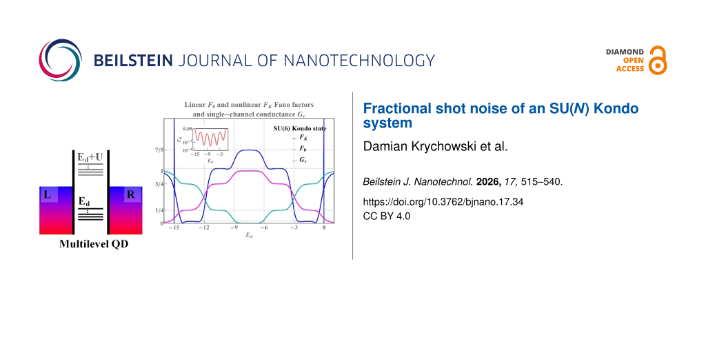
![[2190-4286-17-34-1]](/bjnano/content/figures/2190-4286-17-34-1.png?scale=2.0&max-width=1024&background=FFFFFF)
Figure 1: Kondo effect with even symmetry SU(N = 2, 4, 6): (a, c, d) linear and nonlinear Fano factors F0(K), single-channel quantum conductance Gν, and Wilson ratio Wνν' − 1 as a function of dot energy Ed for N = 2, 4, 6. (b) Gate-dependent FK compared with nonlinear current and shot noise, rescaled by the square of the Kondo temperature. The insets show numerical and analytical approximation of TK (blue and red dashed lines) (U = 3, Γ = 0.025, T = 0, energies are given in units of W/50).
Figure 1: Kondo effect with even symmetry SU(N = 2, 4, 6): (a, c, d) linear and nonlinear Fano factors F0(K),...
Figure 1b shows the variation of the nonlinear Fano factor FK as a function of the atomic level of the quantum dot Ed for the Kondo state with SU(2) symmetry. In the regions of the empty state 0e and the fully occupied state 2e, the Fano factor reaches the value −1, which is related to the dominant influence of the two-body correlation functions ![[Graphic 58]](/bjnano/content/inline/2190-4286-17-34-i118.svg?max-width=637&scale=1.18182) in cV,ν (see Equation 56). In the region with one electron Q = 1e, FK is 5/3, which is in agreement with literature reports [68,84,93,103,104]. In this area,
in cV,ν (see Equation 56). In the region with one electron Q = 1e, FK is 5/3, which is in agreement with literature reports [68,84,93,103,104]. In this area, ![[Graphic 59]](/bjnano/content/inline/2190-4286-17-34-i119.svg?max-width=637&scale=1.18182) and
and ![[Graphic 60]](/bjnano/content/inline/2190-4286-17-34-i120.svg?max-width=637&scale=1.18182) are close to zero. The three-body correlators, as the odd functions of the gate voltage, change the sign in the region with a single electron. The green and magenta lines in Figure 1b show the values of the nonlinear current normalized by the squared Kondo temperature
are close to zero. The three-body correlators, as the odd functions of the gate voltage, change the sign in the region with a single electron. The green and magenta lines in Figure 1b show the values of the nonlinear current normalized by the squared Kondo temperature ![[Graphic 61]](/bjnano/content/inline/2190-4286-17-34-i121.svg?max-width=637&scale=1.18182) and the shot noise
and the shot noise ![[Graphic 62]](/bjnano/content/inline/2190-4286-17-34-i122.svg?max-width=637&scale=1.18182) . This gives the value of the nonlinear Fano factor FK = e*/e = 5/3. Formally, we can write the nonlinear current IK and its fluctuating part SK (first moment of the current correlator) as a sum of two-body and three-body contributions
. This gives the value of the nonlinear Fano factor FK = e*/e = 5/3. Formally, we can write the nonlinear current IK and its fluctuating part SK (first moment of the current correlator) as a sum of two-body and three-body contributions ![[Graphic 63]](/bjnano/content/inline/2190-4286-17-34-i123.svg?max-width=637&scale=1.18182) and, similarly,
and, similarly, ![[Graphic 64]](/bjnano/content/inline/2190-4286-17-34-i124.svg?max-width=637&scale=1.18182) . Near the triple degeneracy points (equality of SB amplitudes
. Near the triple degeneracy points (equality of SB amplitudes ![[Graphic 65]](/bjnano/content/inline/2190-4286-17-34-i125.svg?max-width=637&scale=1.18182) and
and ![[Graphic 66]](/bjnano/content/inline/2190-4286-17-34-i126.svg?max-width=637&scale=1.18182) ), the current IK changes its sign, and, for IK = 0, the nonlinear Fano factor diverges FK → ±∞. This is characteristic for the transition between the Kondo state and the Coulomb blockade regime. Around this transition region, we observe little negative nonlinear shot noise SK < 0. SK is the nonlinear contribution to the shot noise and it might be negative, but the total value S remains positive. In the empty region and for double occupancy n = 2, the nonlinear noise is positive, but small, SK > 0. There are two pairs of points below and above Ed = 0 and Ed = −U, for which FK is zeroing (Figure 1a,b). Similar behavior is also observed for higher symmetries (Figure 1c,d) (close to Ed = 0 and Ed = −3U or Ed = −5U). For an SU(2) dot near Ed = 0 and Ed = −U, also points of vanishing of current are observed (
), the current IK changes its sign, and, for IK = 0, the nonlinear Fano factor diverges FK → ±∞. This is characteristic for the transition between the Kondo state and the Coulomb blockade regime. Around this transition region, we observe little negative nonlinear shot noise SK < 0. SK is the nonlinear contribution to the shot noise and it might be negative, but the total value S remains positive. In the empty region and for double occupancy n = 2, the nonlinear noise is positive, but small, SK > 0. There are two pairs of points below and above Ed = 0 and Ed = −U, for which FK is zeroing (Figure 1a,b). Similar behavior is also observed for higher symmetries (Figure 1c,d) (close to Ed = 0 and Ed = −3U or Ed = −5U). For an SU(2) dot near Ed = 0 and Ed = −U, also points of vanishing of current are observed (![[Graphic 67]](/bjnano/content/inline/2190-4286-17-34-i127.svg?max-width=637&scale=1.18182) ) (orange dots in Figure 1a). Slightly moving from points
) (orange dots in Figure 1a). Slightly moving from points ![[Graphic 68]](/bjnano/content/inline/2190-4286-17-34-i128.svg?max-width=637&scale=1.18182) ≈ 0, −U current IK changes sign in a narrow range of gate voltage due to the three-body correlations (three-body contributions) to coefficients cV,ν (Figure 1b). Around the SK zeroing points, there is also a change in the sign of the nonlinear contribution to the noise. The giant values of |SK| observed in Figure 1a,c,d can be interpreted according to the accepted terminology as hyper-Poissonian noise [84,95]. Careful insight into Figure 1 reveals that this strong enhancement of FK is due to the occurrence of very small current in these regions. For even symmetries SU(N = 2, 4, 6) at half-fillings, the nonlinear noise factor FK takes the value FK = (8 + N)/(4 + N). The equivalent expression can be found in [83].
≈ 0, −U current IK changes sign in a narrow range of gate voltage due to the three-body correlations (three-body contributions) to coefficients cV,ν (Figure 1b). Around the SK zeroing points, there is also a change in the sign of the nonlinear contribution to the noise. The giant values of |SK| observed in Figure 1a,c,d can be interpreted according to the accepted terminology as hyper-Poissonian noise [84,95]. Careful insight into Figure 1 reveals that this strong enhancement of FK is due to the occurrence of very small current in these regions. For even symmetries SU(N = 2, 4, 6) at half-fillings, the nonlinear noise factor FK takes the value FK = (8 + N)/(4 + N). The equivalent expression can be found in [83].
As mentioned earlier [68,84,93,103], three-body correlations vanish at the e–h symmetric point, and, around it, they are small and change signs. In this region, it is the two-body correlation ![[Graphic 69]](/bjnano/content/inline/2190-4286-17-34-i129.svg?max-width=637&scale=1.18182) that modifies current IK and noise SK. For n = 1, 3 in the SU(4) system FK = 1/3, the noise is reduced and of particular importance there are three-body correlation functions
that modifies current IK and noise SK. For n = 1, 3 in the SU(4) system FK = 1/3, the noise is reduced and of particular importance there are three-body correlation functions ![[Graphic 70]](/bjnano/content/inline/2190-4286-17-34-i130.svg?max-width=637&scale=1.18182) and
and ![[Graphic 71]](/bjnano/content/inline/2190-4286-17-34-i131.svg?max-width=637&scale=1.18182) (Figure 2a). In the Q = 1e, 5e charge regions of the SU(6) system, the linear Fano factor is F0 = 3/4, and, for high voltages, the Fano factor is reduced to FK = 1/20 (sub-Poissonian noise). Again responsible for this behavior are the three-particle correlations
(Figure 2a). In the Q = 1e, 5e charge regions of the SU(6) system, the linear Fano factor is F0 = 3/4, and, for high voltages, the Fano factor is reduced to FK = 1/20 (sub-Poissonian noise). Again responsible for this behavior are the three-particle correlations ![[Graphic 72]](/bjnano/content/inline/2190-4286-17-34-i132.svg?max-width=637&scale=1.18182) dominating in these sectors. In the charge regions Q = 2e, 3e, there is a reversed behavior, increase of F, F0 = 1/3, 0, and FK = 21/20, 7/5, respectively, indicating that the residual quasiparticle interactions in the Kondo system cause the super-Poissonian shot noise. Since the interplay of two- and three-body correlations functions decides about the value of the nonlinear Fano factor (Equation 56–Equation 58), we present in Figure 2a,b the gate dependencies of these correlations for exemplarily chosen even SU(4) and odd SU(3) symmetries. The quantities have been rescaled by the Kondo temperature and its square, respectively (see Equation 46 and Equation 47).
dominating in these sectors. In the charge regions Q = 2e, 3e, there is a reversed behavior, increase of F, F0 = 1/3, 0, and FK = 21/20, 7/5, respectively, indicating that the residual quasiparticle interactions in the Kondo system cause the super-Poissonian shot noise. Since the interplay of two- and three-body correlations functions decides about the value of the nonlinear Fano factor (Equation 56–Equation 58), we present in Figure 2a,b the gate dependencies of these correlations for exemplarily chosen even SU(4) and odd SU(3) symmetries. The quantities have been rescaled by the Kondo temperature and its square, respectively (see Equation 46 and Equation 47). ![[Graphic 73]](/bjnano/content/inline/2190-4286-17-34-i133.svg?max-width=637&scale=1.18182) is an even function of the gate voltage, whereas
is an even function of the gate voltage, whereas ![[Graphic 74]](/bjnano/content/inline/2190-4286-17-34-i134.svg?max-width=637&scale=1.18182) is an odd function with a negligible contribution around the e–h symmetry point. The small peaks visible on the correlators for SU(3) symmetry occur in the region of Coulomb blockade boundaries, similar peaks appear also for other odd symmetries (not presented). As can be seen in the following figures, this feature is reflected in the gate dependencies of other physical quantities for odd symmetries.
is an odd function with a negligible contribution around the e–h symmetry point. The small peaks visible on the correlators for SU(3) symmetry occur in the region of Coulomb blockade boundaries, similar peaks appear also for other odd symmetries (not presented). As can be seen in the following figures, this feature is reflected in the gate dependencies of other physical quantities for odd symmetries.
![[2190-4286-17-34-2]](/bjnano/content/figures/2190-4286-17-34-2.png?scale=2.0&max-width=1024&background=FFFFFF)
Figure 2: Two- and three-body correlators rescaled by TK for SU(4) and SU(3) Kondo states (blue and magenta lines). The parameters used in calculations are the same as in Figure 1.
Figure 2: Two- and three-body correlators rescaled by TK for SU(4) and SU(3) Kondo states (blue and magenta l...
Odd symmetries of Kondo states
Figure 3 shows results for Kondo effects with odd degeneracies (N = 3, 5). The e–h symmetry points in these cases correspond to non-integer occupancies (n = 3/2, n = 5/2), and high conductances at these points are associated with the charge resonances centered at the Fermi level. The dependence of conductance on the gate potential at half-filling is characterized by the occurrence of a peak instead of a plateau as in the case of Kondo resonances. In general, however, at e–h symmetric points, the linear conductance for any value of N, regardless of the type of resonance at the Fermi level, takes the unitary limit. For fillings (n = 1, ..., N − 1), conductance plateaus are observed, which manifest Kondo effects for these occupations. For SU(3) symmetry, the value of conductance for n = 1 is (3/4)(e2/h) and, correspondingly, the total conductance is G = (9/4)(e2/h); interestingly, this is the highest total value in the single-charge sector among SU(N) Kondo systems. The curves of linear Fano factors around half-fillings form deeps with F0 = 0 for e–h symmetric points; in Kondo regions F0, they take the values according to the known relationship ![[Graphic 75]](/bjnano/content/inline/2190-4286-17-34-i135.svg?max-width=637&scale=1.18182) . Wilsons ratios decrease with the increase of N (weaker correlations) and are reduced in the areas of charge fluctuations, but, noteworthily, they still have significant values there. Apart from singularities of FK occurring for IK = 0, that is, points located close to empty (n = 0) or fully occupied regions (n = N), an enhancement of FK near the e–h symmetric point is observed F > 1 (the super-Poissonian noise). For N = 3, n ≈ 3/2 three single-electron states become degenerate with three two-electron states. The probability of the occurrence of pairs of quasiparticles is growing in this region, which is associated with an increase in the probability of backscattering of pairs. For N = 5, similarly as for other cases, the numerically calculated plateaus of Kondo conductance for given charge sectors agree with the formula Gν = (e2/h)sin2[Qν].
. Wilsons ratios decrease with the increase of N (weaker correlations) and are reduced in the areas of charge fluctuations, but, noteworthily, they still have significant values there. Apart from singularities of FK occurring for IK = 0, that is, points located close to empty (n = 0) or fully occupied regions (n = N), an enhancement of FK near the e–h symmetric point is observed F > 1 (the super-Poissonian noise). For N = 3, n ≈ 3/2 three single-electron states become degenerate with three two-electron states. The probability of the occurrence of pairs of quasiparticles is growing in this region, which is associated with an increase in the probability of backscattering of pairs. For N = 5, similarly as for other cases, the numerically calculated plateaus of Kondo conductance for given charge sectors agree with the formula Gν = (e2/h)sin2[Qν].
![[2190-4286-17-34-3]](/bjnano/content/figures/2190-4286-17-34-3.png?scale=2.0&max-width=1024&background=FFFFFF)
Figure 3: Odd SU(3) and SU(5) Kondo effect: (a,b) Gate-dependent F0(K), Gν and Wνν' − 1. Insets show numerical and analytical approximation of TK (blue and red dashed lines) (U = 3, Γ = 0.025, T = 0).
Figure 3: Odd SU(3) and SU(5) Kondo effect: (a,b) Gate-dependent F0(K), Gν and Wνν' − 1. Insets show numerica...
For integer values of charge, the Wilson ratio is Wνν' − 1 = 1/4, and, at the boundaries of charge sectors, it is Wνν' − 1 = 1/5. For occupancies n = 1,4, that is, for ranges close to the empty or fully occupied regions, the probability of occurrence of pairs is low, and the backscattering of pairs weakens so much that the nonlinear Fano coefficient FK = 1/5 becomes smaller than the linear noise factor F0 = 2/3. For higher occupancies n = 2,3, pairs of quasiparticles are starting to play a significant role and, as we have checked numerically, both pair correlation functions ![[Graphic 76]](/bjnano/content/inline/2190-4286-17-34-i136.svg?max-width=637&scale=1.18182) and nonlinear correlations
and nonlinear correlations ![[Graphic 77]](/bjnano/content/inline/2190-4286-17-34-i137.svg?max-width=637&scale=1.18182) significantly contribute to the nonlinear noise; FK in this range reaches the value FK = 5/4 and dominates the linear noise (F0 = 1/8).
significantly contribute to the nonlinear noise; FK in this range reaches the value FK = 5/4 and dominates the linear noise (F0 = 1/8).
Equilibrium versus non-equilibrium noise
Figure 4a illustrates voltage dependencies of the total Fano factor F(V/V*) for the exemplarily chosen filling n = 1 (the characteristic value V* is defined in Appendix A). In the linear regime, Fano factors F0 depend only on symmetry and they increase with the increase of degeneracy. This tendency reflects the increasing shift of the Kondo resonance from the Fermi level with the growth of N. For N = 2,3, where residual interactions are stronger than for higher degeneracies, one observes the increase of F with voltage and its saturation for high values of V, F = 5/3, 15/22, respectively. For N ≥ 4, F at high voltages tends to very small values F → 1/3, 0.316, 1/20 for N = 4, 5, 6, respectively. These limits are solely determined by symmetry, which Equation 59 directly shows. In this equation, |F| depends on the degeneracy N, and the Wilson ratio, which is directly related to symmetry Wνν' = 1 + 1/(N − 1).
![[2190-4286-17-34-4]](/bjnano/content/figures/2190-4286-17-34-4.png?scale=2.0&max-width=1024&background=FFFFFF)
Figure 4:
(a) Total Fano factor |F| versus V/V* for SU(N) Kondo states (Q = 1e). (b) Nonlinear Fano factor FK as a function of degeneracy number N for Q = 1e, 3e, 8e (Γ = 0.025, V/V* = 10). The inset compares ![[Graphic 78]](/bjnano/content/inline/2190-4286-17-34-i138.svg?max-width=637&scale=1.18182) and
and ![[Graphic 79]](/bjnano/content/inline/2190-4286-17-34-i139.svg?max-width=637&scale=1.18182) with an increase of N (blue and red lines, Q = 1e). The area filled in red indicates SK < 0. (c,d) FK as a function of Ed and bias-dependent |F| for the SU(4) Kondo state (U = 3, T = 0). TK1 and TK2 in Figure (d) represent two Kondo temperatures for V = 0.
with an increase of N (blue and red lines, Q = 1e). The area filled in red indicates SK < 0. (c,d) FK as a function of Ed and bias-dependent |F| for the SU(4) Kondo state (U = 3, T = 0). TK1 and TK2 in Figure (d) represent two Kondo temperatures for V = 0.
Figure 4: (a) Total Fano factor |F| versus V/V* for SU(N) Kondo states (Q = 1e). (b) Nonlinear Fano factor FK...
Figure 4b compares the dependencies of the nonlinear Fano factor on the rank of the SU(N) group for the selected occupancies. FK > 1 indicates the dominance of bunching processes. This occurs for Q = N/2. In the systems with a larger number of electrons, the ranges in which quasiparticle grouping processes dominate (FK > 1) shift to higher degenerations (N) (Figure 4b). For N = 3, the noise lowers |SK| < 2e|IK|. For N = 7, the influence of three-particle correlation becomes dominant ![[Graphic 80]](/bjnano/content/inline/2190-4286-17-34-i140.svg?max-width=637&scale=1.18182) , which consequently leads to negative noise (SK < 0, inset of Figure 4b). For Q = 3e and 8e, and degenerations N = 3 and N = 8, the nonlinear Fano factor takes the value FK = −1, because two-particle effects in the current dominate there and IK < 0. Interesting to note are the formation of a maximum for N = 6 (Q = 3e) and two maxima for Q = 8e (N = 13, 23). These effects have no fundamental cause; they occur only due to the trigonometric functional dependencies of the phase shifts 2δν and 4δν in the nonlinear noise coefficient (see Equation 57). The nonlinear contribution to noise (Equation 59) leads to FK = −1 in the limit N → ∞ (Figure 4b).
, which consequently leads to negative noise (SK < 0, inset of Figure 4b). For Q = 3e and 8e, and degenerations N = 3 and N = 8, the nonlinear Fano factor takes the value FK = −1, because two-particle effects in the current dominate there and IK < 0. Interesting to note are the formation of a maximum for N = 6 (Q = 3e) and two maxima for Q = 8e (N = 13, 23). These effects have no fundamental cause; they occur only due to the trigonometric functional dependencies of the phase shifts 2δν and 4δν in the nonlinear noise coefficient (see Equation 57). The nonlinear contribution to noise (Equation 59) leads to FK = −1 in the limit N → ∞ (Figure 4b).
The inset in Figure 4b shows nonlinear current and noise as functions of N, scaled by TK for Q = 1e. The calculations were performed for a voltage value of V/V* = 10. In this range, ![[Graphic 81]](/bjnano/content/inline/2190-4286-17-34-i141.svg?max-width=637&scale=1.18182) , the negative value of the noise is close to the nonlinear value of the current and, therefore, FK = −1 (area shaded in red for N > = 7, inset Figure 4b). For N = 2, super-Poissonian processes are dominant; consequently,
, the negative value of the noise is close to the nonlinear value of the current and, therefore, FK = −1 (area shaded in red for N > = 7, inset Figure 4b). For N = 2, super-Poissonian processes are dominant; consequently, ![[Graphic 82]](/bjnano/content/inline/2190-4286-17-34-i142.svg?max-width=637&scale=1.18182) (inset Figure 4b), when N > 2, there is a reversal of the trend
(inset Figure 4b), when N > 2, there is a reversal of the trend ![[Graphic 83]](/bjnano/content/inline/2190-4286-17-34-i143.svg?max-width=637&scale=1.18182) . This is due to the increase of the number of three-particle correlators, which grows with the number of quantum channels. In the case of Q = 1e, it happens for N > = 7.
. This is due to the increase of the number of three-particle correlators, which grows with the number of quantum channels. In the case of Q = 1e, it happens for N > = 7.
Figure 4c,d shows the effect of the coupling strength Γ on |F|. An increase of Γ increases the Kondo temperature (vertical dashed lines in Figure 4d). It causes also a departure from the strictly unitary limits of the SU(4) Kondo effect, that is, from F0 = 1/2 and FK = 1/3. The strongest modification occurs for Q = 1e, 3e, where the charge boundaries 1e/0e and 3e/4e are closest. The region is broadened due to the three-particle correlations. For half-filling, we observe a slight deviation from the value FK = 3/2 due to a slight drop of the Wilson ratio Wνν' = 4/3.
The density maps in Figure 5 show the Fano factor F as a function of V and Ed for the symmetries SU(4) and SU(3). We observe an oscillating line, around V ≈ V*, separating the linear region F0 from the nonlinear Fano factor FK. This line corresponds to the characteristic voltage V* = ![[Graphic 84]](/bjnano/content/inline/2190-4286-17-34-i144.svg?max-width=637&scale=1.18182) ≈ TK, where the slope saturates up to FK. For V > V* the picture of non-interacting Kondo particles falls down, and nonlinear current and shot noise are significant (see Appendices A and D).
≈ TK, where the slope saturates up to FK. For V > V* the picture of non-interacting Kondo particles falls down, and nonlinear current and shot noise are significant (see Appendices A and D).
![[2190-4286-17-34-5]](/bjnano/content/figures/2190-4286-17-34-5.jpg?scale=2.0&max-width=1024&background=FFFFFF)
Figure 5: Density plots of gate-dependent total Fano factor |F| as function of bias voltage V for (a) SU(4) and (b) SU(3) Kondo states (U = 3, Γ = 0.025, T = 0). ±1 indicates the sign of the Fano factor.
Figure 5: Density plots of gate-dependent total Fano factor |F| as function of bias voltage V for (a) SU(4) a...
For the SU(4) Kondo state, regions 1e and 3e show the change from F0 = 1/2 (orange sector) to |FK| = 1/3 (yellow sector) (Figure 5a). In the case of half-filling Q = N/2 = 2e, there is a transition from |F| = F0 = 0 up to |F| = |FK| = 3/2. For SU(3), the balance of two-body (![[Graphic 85]](/bjnano/content/inline/2190-4286-17-34-i145.svg?max-width=637&scale=1.18182) ) and three-body correlations (
) and three-body correlations (![[Graphic 86]](/bjnano/content/inline/2190-4286-17-34-i146.svg?max-width=637&scale=1.18182) ) in shot noise reverses the trend, in this case F0 = 1/4 (yellow sector) and FK ≈ 0.68 (magenta sector) (Figure 5b). This opposite behavior in the case of these two symmetries is explained by Figure 2, where we see that, for SU(4),
) in shot noise reverses the trend, in this case F0 = 1/4 (yellow sector) and FK ≈ 0.68 (magenta sector) (Figure 5b). This opposite behavior in the case of these two symmetries is explained by Figure 2, where we see that, for SU(4), ![[Graphic 87]](/bjnano/content/inline/2190-4286-17-34-i147.svg?max-width=637&scale=1.18182) , whereas, for the SU(3) symmetry,
, whereas, for the SU(3) symmetry, ![[Graphic 88]](/bjnano/content/inline/2190-4286-17-34-i148.svg?max-width=637&scale=1.18182) . The second important result is the transition from F = +1 to F = −1 for the empty and fully occupied states, where the total current is suppressed at the boundary (I = 0, bright white horizontal line). In the region where FK dominates, we observe a characteristic vertical white line; along this line, the nonlinear current vanishes IK = 0. This white line is surrounded by a zeroing contour of nonlinear noise SK = 0 (black envelopes at the boundaries 1e/0e and (N − 1)e/Ne).
. The second important result is the transition from F = +1 to F = −1 for the empty and fully occupied states, where the total current is suppressed at the boundary (I = 0, bright white horizontal line). In the region where FK dominates, we observe a characteristic vertical white line; along this line, the nonlinear current vanishes IK = 0. This white line is surrounded by a zeroing contour of nonlinear noise SK = 0 (black envelopes at the boundaries 1e/0e and (N − 1)e/Ne).
Susceptibility and entropy
Generalized spin susceptibility and entropy provide direct, thermodynamic evidence for the formation of a Kondo singlet. Figure 6 and Figure 7 present the temperature dependencies of susceptibilities, generalized moments, and entropies for different SU(N) systems and various occupancies. TχN (dark curves in Figure 6), where ![[Graphic 89]](/bjnano/content/inline/2190-4286-17-34-i149.svg?max-width=637&scale=1.18182) denotes the generalized spin susceptibility, illustrates the fluctuation with increase of the temperature of the squared generalized SU(N) spins defined by Equation 16. Local Coulomb repulsion favors single occupancies of spin-orbitals, and local SU(N) moments form at high temperatures. This fact is illustrated by the saturation of the continuous lines TχN in Figure 6a–c to the values of squared generalized local SU(N) spins TχN = (N + 1)NQν(1 − Qν)/2. The saturation values are described by Equation 19. For SU(2) and n = 1, the corresponding value is 3/4, for SU(3) 4/3, for SU(4) 15/8, for SU(5) 12/5, and 35/12 for SU(6). Similarly, for n = 2 and n = 3, the saturation values can be read from Figure 6b,c.
denotes the generalized spin susceptibility, illustrates the fluctuation with increase of the temperature of the squared generalized SU(N) spins defined by Equation 16. Local Coulomb repulsion favors single occupancies of spin-orbitals, and local SU(N) moments form at high temperatures. This fact is illustrated by the saturation of the continuous lines TχN in Figure 6a–c to the values of squared generalized local SU(N) spins TχN = (N + 1)NQν(1 − Qν)/2. The saturation values are described by Equation 19. For SU(2) and n = 1, the corresponding value is 3/4, for SU(3) 4/3, for SU(4) 15/8, for SU(5) 12/5, and 35/12 for SU(6). Similarly, for n = 2 and n = 3, the saturation values can be read from Figure 6b,c.
![[2190-4286-17-34-6]](/bjnano/content/figures/2190-4286-17-34-6.png?scale=2.0&max-width=1024&background=FFFFFF)
Figure 6: (a–c) Generalized spin TχN and (TK + T)χN versus T/TK (dark and light lines). The insets illustrate temperature dependencies of isolated and screened SU(4) spin for Q = 1e and Q = 2e, respectively (blue and green lines) (U = 3, Γ = 0.025, V = 0).
Figure 6: (a–c) Generalized spin TχN and (TK + T)χN versus T/TK (dark and light lines). The insets illustrate...
![[2190-4286-17-34-7]](/bjnano/content/figures/2190-4286-17-34-7.png?scale=2.0&max-width=1024&background=FFFFFF)
Figure 7: (a–c) The impurity entropies SN versus T/TK for selected charge regions Q = 1e, 2e, 3e. The insets present temperature-dependent entropy SN=4 of isolated and screened SU(4) impurities (blue and green lines) (U = 3, Γ = 0.025, V = 0).
Figure 7: (a–c) The impurity entropies SN versus T/TK for selected charge regions Q = 1e, 2e, 3e. The insets ...
The light lines in Figure 6 show temperature dependencies of SU(N) susceptibilities. As it is seen, they evolve from Curie-type behavior for high temperatures to Pauli-like behavior, temperature-independent at low temperatures [107]. For example, we show in the insets of Figure 6a,b the exemplary comparison in a wide temperature range of the moments for an isolated SU(4) system (blue lines) with the moments of an SU(4) QD coupled to electrodes (green lines). Around T ∼ ![[Graphic 90]](/bjnano/content/inline/2190-4286-17-34-i150.svg?max-width=637&scale=1.18182) , there is a transition from the range of local moment on the dot to the free-orbital regime, where probability of occupation of all spin-orbitals is equal [108-110]. At low temperatures, below TK, the role of Kondo fluctuations becomes dominant, and, for T → 0, the moment of the dot is dynamically screened by electrode electrons and a many-body SU(N) Kondo singlet is formed. Apart from observations in transport, quite recently also the progressive screening of the spin of a single Anderson impurity (SU(2)) was directly measured [107].
, there is a transition from the range of local moment on the dot to the free-orbital regime, where probability of occupation of all spin-orbitals is equal [108-110]. At low temperatures, below TK, the role of Kondo fluctuations becomes dominant, and, for T → 0, the moment of the dot is dynamically screened by electrode electrons and a many-body SU(N) Kondo singlet is formed. Apart from observations in transport, quite recently also the progressive screening of the spin of a single Anderson impurity (SU(2)) was directly measured [107].
Examples of the temperature dependence of the moments for SU(4) symmetry are illustrated by solid (green) lines in Figure 6a,b. They tend to zero for T → 0. For high temperatures, moments saturate to a value TχN=4 = 15/8. In this specific case, spin σ, orbital moment τ, and multipole στ are also quenched. In general, however, the screening of the SU(N) moment is not necessarily accompanied by quenching of conventional spin or orbital moments. This is the case, for example, for the discussed SU(3) or SU(5) symmetries. Thermodynamic behavior of SU(N) moments coupled to electrode electrons is also reflected in the temperature dependencies of entropy SN. The Kondo ground state is a singlet; therefore, as it is seen in Figure 7, for T → 0, SN → 0. The rise of temperature causes an increase of entropy. For T > TK, the local moment becomes unscreened and free; for n = 1, the entropy is determined by N lowest, degenerate single electron states, and SN = kBln[N]. For n = 2, the low-temperature entropy is determined by the lowest degenerate two-particle states and, for n = 3, by the degenerate three-particle states. Entropy expressed by the slave boson amplitudes is ![[Graphic 91]](/bjnano/content/inline/2190-4286-17-34-i151.svg?max-width=637&scale=1.18182) . For even higher temperatures, more states become excited, allowing thermal energy to be more widely spread. For T ≫
. For even higher temperatures, more states become excited, allowing thermal energy to be more widely spread. For T ≫ ![[Graphic 92]](/bjnano/content/inline/2190-4286-17-34-i152.svg?max-width=637&scale=1.18182) , all N2 states of the SU(N) system are thermally accessible, and entropy reaches the value 2kBln[N]. Examples of entropies in a wide temperature range are presented in the insets of Figure 7a,b.
, all N2 states of the SU(N) system are thermally accessible, and entropy reaches the value 2kBln[N]. Examples of entropies in a wide temperature range are presented in the insets of Figure 7a,b.
Conclusion
We have investigated transport and thermodynamic properties of a multilevel degenerate QD symmetrically coupled to leads. In the analysis of correlations, we innovatively combine the description of the equilibrium Kondo state based on generalized slave boson techniques (SBMFA) with a microsopic Fermi liquid approach for high voltages, the parameters of which were derived from slave boson fields. Our study is the first systematic discussion of all SU(N) Kondo states to high orders up to N = 6. We put special attention on the analysis of the shot noise. Compared to the conductance, shot noise is more difficult to investigate experimentally, but its examination is essential because it provides extended information about dynamics of electron transfer and correlations. The systems under investigations are characterized by the SU(N) group. For N > 2, spin is replaced by generalized spin, which refers to the representation of the SU(N) Lie group. The square of the SU(N) spin, S2, and its longitudinal component SZ commute with the Hamiltonian; hence, the invariant subspaces can by classified by the quantum numbers S and SZ. For even N, many-body resonances appearing in the particle–hole symmetric point of SU(N) structures represent Kondo states, while, for odd N, these are charge resonances. For half-filling, both types of resonances are centered at the Fermi level; therefore, perfect transmission occurs, the partial conductance G reaches the unitary limit at low temperatures (G = e2/h), and the total conductance is G = Ne2/h. The linear Fano factor, also directly related to transmission, vanishes at EF in this case. For this occupancy, the Kondo temperature reaches its lowest value. For even N, Kondo resonances hardly move with the change of gate voltage, and, hence, plateaus are observed in the dependencies of conduction and Fano factors on the gate voltage. For odd N, charge resonances broaden and shift already for small changes of gate voltage, and peaks of conductance or dips of linear Fano factor are seen. The Kondo resonances away from half-filling are shifted relative to the Fermi level; hence, the transmissions decrease and, consequently, the values of conduction plateaus decrease and, correspondingly, F0 plateaus rise. Also, a decrease of TK is observed for n ≠ N/2. Important information is the strength of correlations and, therefore, we also discussed Wilson ratio Wνν', which quantifies it. If this ratio is different from 1, it indicates that the correlations are significant. In Kondo systems, where localized electrons interact strongly with conduction electrons, the Wilson ratio can be enhanced compared to the Fermi gas value. This enhancement is associated with strong fluctuations of the generalized spin and the formation of a Kondo resonance. In the Kondo regime, charge susceptibility in the limit U → ∞ is zero or almost zero for strong interactions; thus, Wilson ratios take the universal values characteristic for a given N and weakly depend on the occupation sector. Interestingly, Wνν' decrease in charge fluctuation regions, but they still retain significant values, indicating the importance of correlations also in these areas. The strength of correlations in a system tends to decrease as the degree of degeneracy increases because more degenerate states allow for compensatory changes to disturbances introduced by interactions. In the limit N → ∞, the quasiparticles become independent, Wνν' → 1. Approaching empty or fully occupied regions, the Wilson ratios also tend to unity for any N.
Screening of magnetic moment by conduction electrons is a key process of the spin-Kondo effect. In this paper we have considered a more general case, the effects of strong coupling of N-dimensional generalized spin with conduction electrons. To illustrate quenching of the generalized moments, we plotted generalized susceptibilities and entropies for each of the examined symmetries. As the temperature is lowered, the susceptibility becomes Pauli-like and temperature-independent, and the effective moment tends to zero. In the Kondo states, the entropy associated with the localized moment is reduced due to the formation of a Kondo singlet resulting from screening of the SU(N) spin. Above T > TK, the entropy reaches SN = kBln[N!/(n!(N − n)!)], and for T = 0 it vanishes. Shot noise measures out-of-equilibrium current fluctuations. As we mentioned earlier in the text, the linear Fano factor corresponds to partition noise, that is, it reflects fluctuations related to the partition of the scattered particles. Nonlinear shot noise arises from the fluctuations in the number of discrete charge carriers passing through a system. It results from interactions between quasiparticles. The important thing is that nonlinear shot noise contains signatures of 2e scattering, which are not seen in the conductance. Our study confirms a conviction of previous authors [82] that taking into account the nonlinear contribution can completely change the picture of fluctuations, in particular whether they are super-Poissonian in nature or sub-Poissonian. These characteristics have been studied by us based on the Fermi liquid theory, assuming dressed, non-interacting pseudofermions defined within SBMFA as quasiparticles. Fermi liquid parameters describing quasiparticle interaction were expressed by two- and three-body correlation functions. Competition of these correlations going beyond linear contribution to the shot noise can determine the nature of nonlinear noise. The dominance of particular scattering processes changes as the energy or chemical potential moves away from the symmetry point. We illustrated on the example of the SU(4) group the general properties of correlations; the two-body correlations are symmetric, whereas three-body correlations are antisymmetric with respect to electron–hole symmetry point. This behavior is a consequence of the fermion nature of particles and the related antisymmetry of the wave functions. Consequently, the three-body residual interactions have a different impact on the behavior of electrons and holes. The three-body correlations vanish at the e–h symmetric point and are very weak in its neighborhood; their absolute value is significant in the Kondo regions beyond half-filling. In contrast, the two-body correlations are positive and dominate for n = N/2; they get weaker away from half-filling so that three-particle residual interactions dominate over two-particle interactions for regions with distinct differences in number of electrons and holes. Our calculations point out that the nonlinear Fano factor tends to decrease with increasing distance from the e–h symmetry point. The current fluctuations of carriers with dominant population become more correlated with the total current, while those of the remaining carriers become less correlated. This leads to less noisy current flow. The rank of the unitary group has also a significant impact on nonlinear shot noise. Higher-symmetry Kondo states tend to have increased shot noise compared to lower-symmetry states due to enhanced many-body correlations involving more components of generalized spin.
The conclusions drawn in this paper can be easily adopted for the case of other structures described by the same Hamiltonian, for example, degenerate impurities, materials with multiple valleys, or cold-atom arrangements. Apart from enriching the knowledge about correlations, the discussed problems are of importance for quantum computing and other quantum technologies. The multidimensional generalized spin (qudit) offers greater information capacity and algorithmic efficiency compared to traditional spins. The Kondo effect provides a powerful, tunable platform to observe and control entanglement. Operating qudit involves carefully tuning the system (e.g., by magnetic or electric fields) to be near or far from the Kondo regime, depending on the desired operation (e.g., initialization, entanglement, or readout). The main limitation of the possible applications of the ordinary spin-SU(2) Kondo effect in nanoobjects is its ultralow Kondo temperature. The increase of SU(N) symmetry removes this problem because TK is growing exponentially with N, and higher temperatures open up possibilities for the practical use of these systems. Noise is a key area of interest. By studying changes in the shot noise, researchers can infer the level of decoherence occurring within the quantum system. This knowledge is extremely important because decoherence is a critical factor that affects the stability and reliability of quantum information.
Appendix A. Slave Boson Formulation
For the discussion of correlation effects, we use the generalized finite-U slave boson mean-field approximation (SBMFA) of Kotliar and Ruckenstein (K-R) [87]. We present here only the basics of the slave boson formalism using a system with N = 6 levels as an example. For lower multiciplicities (N < 6), the formalism is analogous, but simplified due to the smaller number of describes states, which allows for the use of fewer bosons. This reduces the number of self-consistent minimization equations. For SU(6), we introduce a set of boson operators for each electronic configuration of the system. The auxiliary bosons {e, p, d, t, f, q, s} project onto empty, single, double, triple, fourfold, fivefold, and fully occupied states. The single occupation projectors piσ (qiσ) are labeled by orbital or site and spin numbers. Among double (di,dijσσ') and fourfold (fi,fijσ) occupancy bosons, two classes can be distinguished. The first corresponds to the occupancy of a single orbital by two electrons (di) or two holes (fi), and the second describes the double occupancy of electrons (dijσσ') or holes (fijσσ') in different orbitals. The three-electron occupations are represented by twelve bosons (tijσ) corresponding to double occupation of one of the orbitals and single occupation of another, and eight (tσσ'σ'') project onto states with single occupation on the orbital. For SU(6) symmetry, the use of seven independent slave bosonic (SB) operators is sufficient; in general, for SU(N), their number is (N + 1). Apart from slave bosonic operators, one also introduces in the SB approach auxiliary fermionic operators, in terms of which the physical electron operators diσ are expressed by ziσfiσ, where ziσ is the transfer bosonic like-operator, which modifies coupling to the leads:
![[2190-4286-17-34-i25]](/bjnano/content/inline/2190-4286-17-34-i25.svg?max-width=590&scale=1.18182)
fiσ represents the pseudo-fermionic operators that renormalize orbital–lead hybridization, ![[Graphic 93]](/bjnano/content/inline/2190-4286-17-34-i153.svg?max-width=637&scale=1.18182) is the square of the orbital-spin fluctuations number, and
is the square of the orbital-spin fluctuations number, and
![[2190-4286-17-34-i26]](/bjnano/content/inline/2190-4286-17-34-i26.svg?max-width=590&scale=1.18182)
denotes the charge operator. The tunneling (transfer) operator ![[Graphic 94]](/bjnano/content/inline/2190-4286-17-34-i154.svg?max-width=637&scale=1.18182) is normalized by the variance of orbital-spin occupancy number
is normalized by the variance of orbital-spin occupancy number ![[Graphic 95]](/bjnano/content/inline/2190-4286-17-34-i155.svg?max-width=637&scale=1.18182) . The above form of effective resonant line narrowing factors ziσ are chosen in order to obtain the correct MFA limit in the uncorrelated case. To eliminate additional unphysical states introduced by SB representation, one supplements the SB Hamiltonian with conditions of charge conservation Qiσ and completeness relation expressed by equating the sum of bosonic amplitudes with the unit operator
. The above form of effective resonant line narrowing factors ziσ are chosen in order to obtain the correct MFA limit in the uncorrelated case. To eliminate additional unphysical states introduced by SB representation, one supplements the SB Hamiltonian with conditions of charge conservation Qiσ and completeness relation expressed by equating the sum of bosonic amplitudes with the unit operator
![[2190-4286-17-34-i27]](/bjnano/content/inline/2190-4286-17-34-i27.svg?max-width=590&scale=1.18182)
These constraints are built into the SB Hamiltonian by introducing Lagrange multipliers λ and λiσ. The corresponding extended K-R Hamiltonian then reads:
![[2190-4286-17-34-i28]](/bjnano/content/inline/2190-4286-17-34-i28.svg?max-width=590&scale=1.18182)
where ![[Graphic 96]](/bjnano/content/inline/2190-4286-17-34-i156.svg?max-width=637&scale=1.18182) is the pseudofermion occupation number operator [87]. The MFA ground state is found using the saddle-point approximation (K-R), in which all boson fields are replaced by their expectation values, found from the condition that
is the pseudofermion occupation number operator [87]. The MFA ground state is found using the saddle-point approximation (K-R), in which all boson fields are replaced by their expectation values, found from the condition that ![[Graphic 97]](/bjnano/content/inline/2190-4286-17-34-i157.svg?max-width=637&scale=1.18182) has an absolute minimum as a function of variables {bn=1..64} = {e, piσ, di, dijσσ', ti,jσ, tσσ'σ'', fi, fijσσ', qiσ, s} and the Lagrange multipliers λ, λiσ. In this way, the problem is formally reduced to the effective quasiparticle model with renormalized hopping integrals and renormalized dot energies. The resulting self-consistent minimization equations read:
has an absolute minimum as a function of variables {bn=1..64} = {e, piσ, di, dijσσ', ti,jσ, tσσ'σ'', fi, fijσσ', qiσ, s} and the Lagrange multipliers λ, λiσ. In this way, the problem is formally reduced to the effective quasiparticle model with renormalized hopping integrals and renormalized dot energies. The resulting self-consistent minimization equations read:
![[2190-4286-17-34-i29]](/bjnano/content/inline/2190-4286-17-34-i29.svg?max-width=590&scale=1.18182)
where
![[2190-4286-17-34-i30]](/bjnano/content/inline/2190-4286-17-34-i30.svg?max-width=590&scale=1.18182)
![[Graphic 98]](/bjnano/content/inline/2190-4286-17-34-i158.svg?max-width=637&scale=1.18182)
![[Graphic 99]](/bjnano/content/inline/2190-4286-17-34-i159.svg?max-width=637&scale=1.18182)
![[Graphic 100]](/bjnano/content/inline/2190-4286-17-34-i160.svg?max-width=637&scale=1.18182)
![[Graphic 101]](/bjnano/content/inline/2190-4286-17-34-i161.svg?max-width=637&scale=1.18182)
![[Graphic 102]](/bjnano/content/inline/2190-4286-17-34-i162.svg?max-width=637&scale=1.18182) correspond to effective corrections of the dot energies for different occupations. The correlators can be expressed by the corresponding non-equilibrium Green’s functions:
correspond to effective corrections of the dot energies for different occupations. The correlators can be expressed by the corresponding non-equilibrium Green’s functions:
![[2190-4286-17-34-i31]](/bjnano/content/inline/2190-4286-17-34-i31.svg?max-width=590&scale=1.18182)
![[Graphic 103]](/bjnano/content/inline/2190-4286-17-34-i163.svg?max-width=637&scale=1.18182) are the non-equilibrium Green’s functions that can be found by the equations-of-motion method applied to the SB Hamiltonian (Equation 2).
are the non-equilibrium Green’s functions that can be found by the equations-of-motion method applied to the SB Hamiltonian (Equation 2). ![[Graphic 104]](/bjnano/content/inline/2190-4286-17-34-i164.svg?max-width=637&scale=1.18182) and
and ![[Graphic 105]](/bjnano/content/inline/2190-4286-17-34-i165.svg?max-width=637&scale=1.18182) are, respectively, lesser and advanced self-energies. The retarded and advanced Green’s functions in channel ν are
are, respectively, lesser and advanced self-energies. The retarded and advanced Green’s functions in channel ν are ![[Graphic 106]](/bjnano/content/inline/2190-4286-17-34-i166.svg?max-width=637&scale=1.18182) , where the poles determine position
, where the poles determine position ![[Graphic 107]](/bjnano/content/inline/2190-4286-17-34-i167.svg?max-width=637&scale=1.18182) and width of the quasiparticle resonance
and width of the quasiparticle resonance ![[Graphic 108]](/bjnano/content/inline/2190-4286-17-34-i168.svg?max-width=637&scale=1.18182) . The corresponding characteristic resonance temperature is
. The corresponding characteristic resonance temperature is ![[Graphic 109]](/bjnano/content/inline/2190-4286-17-34-i169.svg?max-width=637&scale=1.18182) . The renormalized level position and the width also specify the located charge and, thus, also the phase shift (δν) at a given orbital Qν = δν/π. The link between the complex pole of the Green’s function, charge, and characteristic temperature can be expressed as follows [89]:
. The renormalized level position and the width also specify the located charge and, thus, also the phase shift (δν) at a given orbital Qν = δν/π. The link between the complex pole of the Green’s function, charge, and characteristic temperature can be expressed as follows [89]:
![[2190-4286-17-34-i32]](/bjnano/content/inline/2190-4286-17-34-i32.svg?max-width=590&scale=1.18182)
or equivalently:
![[2190-4286-17-34-i33]](/bjnano/content/inline/2190-4286-17-34-i33.svg?max-width=590&scale=1.18182)
In the mean-field approximation, the free energy corresponding to the Hamiltonian in Equation 2 is a sum of slave-boson free energy ![[Graphic 110]](/bjnano/content/inline/2190-4286-17-34-i170.svg?max-width=637&scale=1.18182) and fermionic contribution
and fermionic contribution ![[Graphic 111]](/bjnano/content/inline/2190-4286-17-34-i171.svg?max-width=637&scale=1.18182) (
(![[Graphic 112]](/bjnano/content/inline/2190-4286-17-34-i172.svg?max-width=637&scale=1.18182) ). Using the Matsubara Green’s function the fermionic and bosonic free energies can be written as:
). Using the Matsubara Green’s function the fermionic and bosonic free energies can be written as:
![[2190-4286-17-34-i34]](/bjnano/content/inline/2190-4286-17-34-i34.svg?max-width=590&scale=1.18182)
where ![[Graphic 113]](/bjnano/content/inline/2190-4286-17-34-i173.svg?max-width=637&scale=1.18182) is the full f-electron propagator in the presence of the Bose field (represented by the Green’s function matrix in general), iwn are the Matsubara frequencies, and
is the full f-electron propagator in the presence of the Bose field (represented by the Green’s function matrix in general), iwn are the Matsubara frequencies, and ![[Graphic 114]](/bjnano/content/inline/2190-4286-17-34-i174.svg?max-width=637&scale=1.18182) are the complex poles of the quasiparticle Kondo resonance. After integration of Equation 12 on the complex plane, one gets [111]:
are the complex poles of the quasiparticle Kondo resonance. After integration of Equation 12 on the complex plane, one gets [111]:
![[2190-4286-17-34-i35]](/bjnano/content/inline/2190-4286-17-34-i35.svg?max-width=590&scale=1.18182)
where ![[Graphic 115]](/bjnano/content/inline/2190-4286-17-34-i175.svg?max-width=637&scale=1.18182)
![[Graphic 116]](/bjnano/content/inline/2190-4286-17-34-i176.svg?max-width=637&scale=1.18182) and Ψ0 is the digamma function [89]. The slave boson contribution is:
and Ψ0 is the digamma function [89]. The slave boson contribution is:
![[2190-4286-17-34-i36]](/bjnano/content/inline/2190-4286-17-34-i36.svg?max-width=590&scale=1.18182)
The phase shift δν, which, according to Friedel sum rules, determines the elastic scattering, is linked with the corresponding partial density of states at the Fermi level as follows ![[Graphic 117]](/bjnano/content/inline/2190-4286-17-34-i177.svg?max-width=637&scale=1.18182) . At zero temperature, δν is also related to the occupation number by:
. At zero temperature, δν is also related to the occupation number by:
![[2190-4286-17-34-i37]](/bjnano/content/inline/2190-4286-17-34-i37.svg?max-width=590&scale=1.18182)
Similarly, static two-body susceptibilities ![[Graphic 118]](/bjnano/content/inline/2190-4286-17-34-i178.svg?max-width=637&scale=1.18182)
![[Graphic 119]](/bjnano/content/inline/2190-4286-17-34-i179.svg?max-width=637&scale=1.18182) and three-body correlation functions
and three-body correlation functions ![[Graphic 120]](/bjnano/content/inline/2190-4286-17-34-i180.svg?max-width=637&scale=1.18182) are expressed through derivatives of the free energy with respect to site energies. δnν denote deviations from the ground state distribution δnν ≡ nν − ⟨nν(0)⟩.
are expressed through derivatives of the free energy with respect to site energies. δnν denote deviations from the ground state distribution δnν ≡ nν − ⟨nν(0)⟩.
The diagonal fermionic susceptibilities at low temperatures are given by [89]:
![[2190-4286-17-34-i38]](/bjnano/content/inline/2190-4286-17-34-i38.svg?max-width=590&scale=1.18182)
![[2190-4286-17-34-i39]](/bjnano/content/inline/2190-4286-17-34-i39.svg?max-width=590&scale=1.18182)
where Ψ1(2)(z) are the first and second derivative of the digamma function Ψ0. Equation 38 and Equation 39 determine correlators within the SBMFA approach. Although quasiparticles in this approximation are formally treated as non-interacting, some of the effects of interaction are encoded in this approach by renormalization of parameters.
For discussion of the out-of-equilibrium case (V ≠ 0), we extended the MFA approach to slave bosons by including into the self-consistent minimization equations the free energy supplemented by the Fermi liquid interactions term ![[Graphic 121]](/bjnano/content/inline/2190-4286-17-34-i181.svg?max-width=637&scale=1.18182) (Equation 20). We integrated
(Equation 20). We integrated ![[Graphic 122]](/bjnano/content/inline/2190-4286-17-34-i182.svg?max-width=637&scale=1.18182) putting
putting ![[Graphic 123]](/bjnano/content/inline/2190-4286-17-34-i183.svg?max-width=637&scale=1.18182) and taking the fluctuation of the occupation number δnν =
and taking the fluctuation of the occupation number δnν = ![[Graphic 124]](/bjnano/content/inline/2190-4286-17-34-i184.svg?max-width=637&scale=1.18182)
![[Graphic 125]](/bjnano/content/inline/2190-4286-17-34-i185.svg?max-width=637&scale=1.18182) (fα is the Fermi–Dirac distribution and Θ is the Heaviside function). In this generalized procedure appeared the new additional minimization parameter δEν (fluctuation of energy levels of FL quasiparticles). The corresponding minimization equation is
(fα is the Fermi–Dirac distribution and Θ is the Heaviside function). In this generalized procedure appeared the new additional minimization parameter δEν (fluctuation of energy levels of FL quasiparticles). The corresponding minimization equation is ![[Graphic 126]](/bjnano/content/inline/2190-4286-17-34-i186.svg?max-width=637&scale=1.18182) , and it supplements Equation 29 and Equation 30. As is seen in Figure 8, the SBMFA solutions do not exists for V ≫ TK. The proposed method interpolates slave boson approach for high voltages. This approach extends the existence of auxiliary bosons in the voltage range U ≫ V > TK (Figure 8). This method is an alternative proposition to the problem of fluctuations in FL theory different from the earlier schemes presented, for example, in [90,111,112]. The condition ∂2|F|/∂V2 = 0 determines the characteristic voltage
, and it supplements Equation 29 and Equation 30. As is seen in Figure 8, the SBMFA solutions do not exists for V ≫ TK. The proposed method interpolates slave boson approach for high voltages. This approach extends the existence of auxiliary bosons in the voltage range U ≫ V > TK (Figure 8). This method is an alternative proposition to the problem of fluctuations in FL theory different from the earlier schemes presented, for example, in [90,111,112]. The condition ∂2|F|/∂V2 = 0 determines the characteristic voltage ![[Graphic 130]](/bjnano/content/inline/2190-4286-17-34-i190.svg?max-width=637&scale=1.18182) , for which the picture of non-interacting Kondo particles breaks down and Landauer’s description no longer applies.
, for which the picture of non-interacting Kondo particles breaks down and Landauer’s description no longer applies.
![[2190-4286-17-34-8]](/bjnano/content/figures/2190-4286-17-34-8.png?scale=2.0&max-width=1024&background=FFFFFF)
Figure 8:
Slave boson amplitudes ![[Graphic 127]](/bjnano/content/inline/2190-4286-17-34-i187.svg?max-width=637&scale=1.18182) , d2 and the fluctuation parameter δEν versus bias voltage (magenta dark cyan and black lines). Solid and dashed curves represent, respectively, the self-consistent calculations without and with FL correction (
, d2 and the fluctuation parameter δEν versus bias voltage (magenta dark cyan and black lines). Solid and dashed curves represent, respectively, the self-consistent calculations without and with FL correction (![[Graphic 128]](/bjnano/content/inline/2190-4286-17-34-i188.svg?max-width=637&scale=1.18182) ) to free fermion energy
) to free fermion energy ![[Graphic 129]](/bjnano/content/inline/2190-4286-17-34-i189.svg?max-width=637&scale=1.18182) . TK is shown on the V-axis. Blue line illustrates total |F| versus V for SU(2) Kondo state (U = 3, T = 0, Ed = −U/2, Γ = 0.05).
. TK is shown on the V-axis. Blue line illustrates total |F| versus V for SU(2) Kondo state (U = 3, T = 0, Ed = −U/2, Γ = 0.05).
Figure 8:
Slave boson amplitudes , d2 and the fluctuation parameter δEν versus bias voltage (magenta dark cya...
Appendix B. The Analytical Expression for the Kondo Temperature in the SBMFA Formalism
Here we only sketch the main points of the derivation, a more detailed analysis, but only for the special case of SU(4) symmetry can be found in Appendix A of [113]. We restrict ourselves to the fully symmetric SU(N) Kondo state. In this case, the number of independent boson operators reduces from 2N to N + 1. To derive an approximate analytical formula for TK applicable in a given charge sector {Q} and for simplicity, we take into account the relationship of the minimization Equation 3 for a given charge sector {Q} with analogous equations, but only from the nearest sectors {Q ± 1}. This simplification means that the dynamics within a given charge sector Q = ne is influenced by fluctuations (n − 1)e ↔ ne and ne ↔ (n + 1)e alone. Let us denote the difference of two self-consistent equations for n and n − 1 and for given N by ![[Graphic 131]](/bjnano/content/inline/2190-4286-17-34-i191.svg?max-width=637&scale=1.18182) (N):
(N):
![[2190-4286-17-34-i40]](/bjnano/content/inline/2190-4286-17-34-i40.svg?max-width=590&scale=1.18182)
For V = 0 and T = 0 the above formula is simplified to:
![[2190-4286-17-34-i41]](/bjnano/content/inline/2190-4286-17-34-i41.svg?max-width=590&scale=1.18182)
In the unitary limit, λν ≈ Ed and then:
![[2190-4286-17-34-i42]](/bjnano/content/inline/2190-4286-17-34-i42.svg?max-width=590&scale=1.18182)
and similarly
![[2190-4286-17-34-i43]](/bjnano/content/inline/2190-4286-17-34-i43.svg?max-width=590&scale=1.18182)
where the coefficients ![[Graphic 132]](/bjnano/content/inline/2190-4286-17-34-i192.svg?max-width=637&scale=1.18182) (N) and
(N) and ![[Graphic 133]](/bjnano/content/inline/2190-4286-17-34-i193.svg?max-width=637&scale=1.18182) (N) are assigned to the virtual transitions between neighboring charge states. For N = 2
(N) are assigned to the virtual transitions between neighboring charge states. For N = 2 ![[Graphic 134]](/bjnano/content/inline/2190-4286-17-34-i194.svg?max-width=637&scale=1.18182) = {4,4}, N = 3
= {4,4}, N = 3 ![[Graphic 135]](/bjnano/content/inline/2190-4286-17-34-i195.svg?max-width=637&scale=1.18182) = {6,9/2}, {9/2,6}, and for N = 4 {8,16/3}, {6,6}, {16/3,8}. For SU(5) and SU(6) Kondo symmetries,
= {6,9/2}, {9/2,6}, and for N = 4 {8,16/3}, {6,6}, {16/3,8}. For SU(5) and SU(6) Kondo symmetries, ![[Graphic 136]](/bjnano/content/inline/2190-4286-17-34-i196.svg?max-width=637&scale=1.18182) = {10,25/4}, {15/2,20/3} and {12,36/5}, {9,15/2}, {8,8}, respectively. For infinite U,
= {10,25/4}, {15/2,20/3} and {12,36/5}, {9,15/2}, {8,8}, respectively. For infinite U, ![[Graphic 137]](/bjnano/content/inline/2190-4286-17-34-i197.svg?max-width=637&scale=1.18182) is different from zero, and
is different from zero, and ![[Graphic 138]](/bjnano/content/inline/2190-4286-17-34-i198.svg?max-width=637&scale=1.18182) = N2/(N − 1); in particular, for the SU(4) symmetry,
= N2/(N − 1); in particular, for the SU(4) symmetry, ![[Graphic 139]](/bjnano/content/inline/2190-4286-17-34-i199.svg?max-width=637&scale=1.18182) = 16/3 [113]. Comparing the left sides of Equation 28 and Equation 29 allows us to determine the SU(N) Kondo temperature in selected charge sectors Q = ne.
= 16/3 [113]. Comparing the left sides of Equation 28 and Equation 29 allows us to determine the SU(N) Kondo temperature in selected charge sectors Q = ne.
![[2190-4286-17-34-i44]](/bjnano/content/inline/2190-4286-17-34-i44.svg?max-width=590&scale=1.18182)
From Equation 30 it follows:
![[2190-4286-17-34-i45]](/bjnano/content/inline/2190-4286-17-34-i45.svg?max-width=590&scale=1.18182)
The Kondo temperature is expressed in terms of the bare parameters of the Anderson model. Equation 31 generalizes the K-R SBMFA expression for SU(2) onto the systems of higher symmetries SU(N), N > 2. For infinite U, Equation 31 is simplified to:
![[2190-4286-17-34-i46]](/bjnano/content/inline/2190-4286-17-34-i46.svg?max-width=590&scale=1.18182)
For N = 2, the above formula differs from Coleman’s SBMFA expression [114,115] and from the commonly cited formula for TK derived from Schrieffer–Wolff transformation [24] by a factor of two in the denominator of the exponent. The difference is related to disparate representation of charge fluctuations in the K-R and Coleman approaches (different number of SB operators). For N = 4, Equation 32 has been derived earlier by us [113]. The Kondo temperature increases with an increase of degeneracy. This is most clearly seen in the limit of infinite U, where the Kondo temperature scales by only one coefficient in the standard exponential dependence, namely, ![[Graphic 140]](/bjnano/content/inline/2190-4286-17-34-i200.svg?max-width=637&scale=1.18182) [15,113]. For high degeneracy,
[15,113]. For high degeneracy, ![[Graphic 141]](/bjnano/content/inline/2190-4286-17-34-i201.svg?max-width=637&scale=1.18182) → N. The increase in TK along with the increase in degeneration opens a window to Kondo system applications. The increase of TK with N is observed in differential conductance spectroscopy [11,29,101], where the width of the quasiparticle resonance increases with higher N [15].
→ N. The increase in TK along with the increase in degeneration opens a window to Kondo system applications. The increase of TK with N is observed in differential conductance spectroscopy [11,29,101], where the width of the quasiparticle resonance increases with higher N [15].
We can express two- and three-body correlation functions using the Kondo temperature as follows:
![[2190-4286-17-34-i47]](/bjnano/content/inline/2190-4286-17-34-i47.svg?max-width=590&scale=1.18182)
![[2190-4286-17-34-i48]](/bjnano/content/inline/2190-4286-17-34-i48.svg?max-width=590&scale=1.18182)
Based on the above equations, we find ![[Graphic 142]](/bjnano/content/inline/2190-4286-17-34-i202.svg?max-width=637&scale=1.18182) , and we can write equivalently the Kondo temperature (Equation 31) as a function of not only two-body, but also three-particle, correlators:
, and we can write equivalently the Kondo temperature (Equation 31) as a function of not only two-body, but also three-particle, correlators:
![[2190-4286-17-34-i49]](/bjnano/content/inline/2190-4286-17-34-i49.svg?max-width=590&scale=1.18182)
Appendix C. Susceptibilities and Wilson Ratio of an isolated N-QD
The slave boson Hamiltonian of the N-QD in the atomic limit (t = 0) reads:
![[2190-4286-17-34-i50]](/bjnano/content/inline/2190-4286-17-34-i50.svg?max-width=590&scale=1.18182)
The corresponding partition function is:
![[2190-4286-17-34-i51]](/bjnano/content/inline/2190-4286-17-34-i51.svg?max-width=590&scale=1.18182)
where β = 1/kBT, ![[Graphic 143]](/bjnano/content/inline/2190-4286-17-34-i203.svg?max-width=637&scale=1.18182) and
and ![[Graphic 144]](/bjnano/content/inline/2190-4286-17-34-i204.svg?max-width=637&scale=1.18182) is defined in the main text. The probability distribution can be determined by the assignment:
is defined in the main text. The probability distribution can be determined by the assignment:
![[2190-4286-17-34-i52]](/bjnano/content/inline/2190-4286-17-34-i52.svg?max-width=590&scale=1.18182)
The free energy of an isolated N-QD is F(0) = −(1/β)ln(![[Graphic 145]](/bjnano/content/inline/2190-4286-17-34-i205.svg?max-width=637&scale=1.18182) ). Now, we present formulas for susceptibilities. For clarity and brevity of expressions, we illustrate the derivation of formulas only for the simplest case of SU(2) symmetry, which requires the use of four slave bosons. For higher symmetries, the considerations are completely analogous. For SU(2) symmetry, the set of SB operators is
). Now, we present formulas for susceptibilities. For clarity and brevity of expressions, we illustrate the derivation of formulas only for the simplest case of SU(2) symmetry, which requires the use of four slave bosons. For higher symmetries, the considerations are completely analogous. For SU(2) symmetry, the set of SB operators is ![[Graphic 146]](/bjnano/content/inline/2190-4286-17-34-i206.svg?max-width=637&scale=1.18182) and
and ![[Graphic 147]](/bjnano/content/inline/2190-4286-17-34-i207.svg?max-width=637&scale=1.18182) . Susceptibilities are given by:
. Susceptibilities are given by:
![[2190-4286-17-34-i53]](/bjnano/content/inline/2190-4286-17-34-i53.svg?max-width=590&scale=1.18182)
Using the inverted relation to Equation 42 we can write:
![[2190-4286-17-34-i54]](/bjnano/content/inline/2190-4286-17-34-i54.svg?max-width=590&scale=1.18182)
where ![[Graphic 148]](/bjnano/content/inline/2190-4286-17-34-i208.svg?max-width=637&scale=1.18182) is the charge in state ν and Qνν' =
is the charge in state ν and Qνν' = ![[Graphic 149]](/bjnano/content/inline/2190-4286-17-34-i209.svg?max-width=637&scale=1.18182) is the inter-state charge correlator.
is the inter-state charge correlator.
The Wilson ratio
![[2190-4286-17-34-i55]](/bjnano/content/inline/2190-4286-17-34-i55.svg?max-width=590&scale=1.18182)
can be expressed using Equation 44 as follows:
![[2190-4286-17-34-i56]](/bjnano/content/inline/2190-4286-17-34-i56.svg?max-width=590&scale=1.18182)
It is important to note that, while the corresponding bosonic expressions for the susceptibilities differ for individual symmetries because the sets of auxiliary bosons are different, the formulas for susceptibilities given by the charges and charge correlators have a general form, applying to any N. According to the argument presented in the main text, we adopt the above formula for Wνν' (Equation 44) also for the case when electrodes are weakly linked to the dot (see Equation 18).
Figure 9 presents the dependence of the generalized Wilson ratio on the Coulomb interaction parameter U exemplarily for Q = 1e. For high values of U, Wνν' − 1 saturates and takes the values 1/(N − 1) (inset in Figure 9), which agrees with the results of NRG and perturbation theory calculus [80,84,96]. As we have shown earlier, in the regime of strong coupling, the Wilson coefficient depends only on symmetry (N); due to the smallness of the quasiparticle amplitude ![[Graphic 150]](/bjnano/content/inline/2190-4286-17-34-i210.svg?max-width=637&scale=1.18182) , it is well defined by the charges Qν and the inter-charge correlator Qνν' (Equation 56). Lowering the coupling value with the electrodes Γ effectively shifts the saturation point (N − 1)(Wνν' − 1) toward lower U values.
, it is well defined by the charges Qν and the inter-charge correlator Qνν' (Equation 56). Lowering the coupling value with the electrodes Γ effectively shifts the saturation point (N − 1)(Wνν' − 1) toward lower U values.
![[2190-4286-17-34-9]](/bjnano/content/figures/2190-4286-17-34-9.png?scale=2.0&max-width=1024&background=FFFFFF)
Figure 9: Generalized Wilson ratio (N − 1)(Wνν' − 1) as a function of Coulomb interaction U in the 1e charge region. The inset shows Wνν' − 1 versus U (Γ = 0.05). The green dashed line shows the generalized Wilson ratio of the SU(4) Kondo state for Γ = 0.025. The dashed vertical gray line represents U used in calculations.
Figure 9: Generalized Wilson ratio (N − 1)(Wνν' − 1) as a function of Coulomb interaction U in the 1e charge ...
Appendix D. Nonlinear Shot Noise of FL Quasiparticles in SBMFA
As shown in [82,83], the nonlinear coefficients cV,ν and cS,ν of current and shot noise can be expressed by the following high-order correlations and phase shifts as follows:
![[2190-4286-17-34-i57]](/bjnano/content/inline/2190-4286-17-34-i57.svg?max-width=590&scale=1.18182)
![[2190-4286-17-34-i58]](/bjnano/content/inline/2190-4286-17-34-i58.svg?max-width=590&scale=1.18182)
The nonlinear Fano factor FK reads [82]:
![[2190-4286-17-34-i59]](/bjnano/content/inline/2190-4286-17-34-i59.svg?max-width=590&scale=1.18182)
Expressing two- and three-particle functions in Equation 57 and Equation 58 by slave-boson mean-field correlators, we can rewrite the total shot noise formula for SU(N) Kondo quasiparticles up to V3 as follows:
![[2190-4286-17-34-i60]](/bjnano/content/inline/2190-4286-17-34-i60.svg?max-width=590&scale=1.18182)
Equation 60 explicitly shows the dependence of |F| on Kondo resonance characteristics (![[Graphic 151]](/bjnano/content/inline/2190-4286-17-34-i211.svg?max-width=637&scale=1.18182) and
and ![[Graphic 152]](/bjnano/content/inline/2190-4286-17-34-i212.svg?max-width=637&scale=1.18182) ), degeneracy (N), and Wilson ratio Wνν'. When Wνν' = 1, the interaction corrections disappear, and the system behaves like a noninteracting system of Kondo particles.
), degeneracy (N), and Wilson ratio Wνν'. When Wνν' = 1, the interaction corrections disappear, and the system behaves like a noninteracting system of Kondo particles.
Data Availability Statement
All data that supports the findings of this study is available in the published article and/or the supporting information of this article.
References
-
Petta, J. R.; Johnson, A. C.; Taylor, J. M.; Laird, E. A.; Yacoby, A.; Lukin, M. D.; Marcus, C. M.; Hanson, M. P.; Gossard, A. C. Science 2005, 309, 2180–2184. doi:10.1126/science.1116955
Return to citation in text: [1] -
Elzerman, J. M.; Hanson, R.; Willems van Beveren, L. H.; Witkamp, B.; Vandersypen, L. M. K.; Kouwenhoven, L. P. Nature 2004, 430, 431–435. doi:10.1038/nature02693
Return to citation in text: [1] -
Loss, D.; DiVincenzo, D. P. Phys. Rev. A 1998, 57, 120–126. doi:10.1103/physreva.57.120
Return to citation in text: [1] -
Kouwenhoven, L.; Glazman, L. Phys. World 2001, 14, 33–38. doi:10.1088/2058-7058/14/1/28
Return to citation in text: [1] [2] -
Goldhaber-Gordon, D.; Shtrikman, H.; Mahalu, D.; Abusch-Magder, D.; Meirav, U.; Kastner, M. A. Nature 1998, 391, 156–159. doi:10.1038/34373
Return to citation in text: [1] [2] [3] -
Cronenwett, S. M.; Oosterkamp, T. H.; Kouwenhoven, L. P. Science 1998, 281, 540–544. doi:10.1126/science.281.5376.540
Return to citation in text: [1] [2] [3] -
Makarovski, A.; Zhukov, A.; Liu, J.; Finkelstein, G. Phys. Rev. B 2007, 75, 241407. doi:10.1103/physrevb.75.241407
Return to citation in text: [1] [2] [3] [4] [5] -
Lim, J. S.; Choi, M.-S.; Choi, M. Y.; López, R.; Aguado, R. Phys. Rev. B 2006, 74, 205119. doi:10.1103/physrevb.74.205119
Return to citation in text: [1] [2] -
Laird, E. A.; Kuemmeth, F.; Steele, G. A.; Grove-Rasmussen, K.; Nygård, J.; Flensberg, K.; Kouwenhoven, L. P. Rev. Mod. Phys. 2015, 87, 703–764. doi:10.1103/revmodphys.87.703
Return to citation in text: [1] -
Krychowski, D.; Lipiński, S. Eur. Phys. J. B 2018, 91, 8. doi:10.1140/epjb/e2017-80547-y
Return to citation in text: [1] [2] -
Nygård, J.; Cobden, D. H.; Lindelof, P. E. Nature 2000, 408, 342–346. doi:10.1038/35042545
Return to citation in text: [1] [2] -
Park, J.; Pasupathy, A. N.; Goldsmith, J. I.; Chang, C.; Yaish, Y.; Petta, J. R.; Rinkoski, M.; Sethna, J. P.; Abruña, H. D.; McEuen, P. L.; Ralph, D. C. Nature 2002, 417, 722–725. doi:10.1038/nature00791
Return to citation in text: [1] -
Liang, W.; Shores, M. P.; Bockrath, M.; Long, J. R.; Park, H. Nature 2002, 417, 725–729. doi:10.1038/nature00790
Return to citation in text: [1] -
Kondo, J. Prog. Theor. Phys. 1964, 32, 37–49. doi:10.1143/ptp.32.37
Return to citation in text: [1] -
Hewson, A. C. The Kondo Problem to Heavy Fermions; Cambridge University Press: Cambridge, 1993. doi:10.1017/cbo9780511470752
Return to citation in text: [1] [2] [3] [4] [5] [6] -
Yoo, G.; Lee, S.-S. B.; Sim, H.-S. Phys. Rev. Lett. 2018, 120, 146801. doi:10.1103/physrevlett.120.146801
Return to citation in text: [1] -
Xing, Y.; Chen, H.; Hu, B.; Ye, Y.; Hofer, W. A.; Gao, H.-J. Nano Res. 2022, 15, 1466–1471. doi:10.1007/s12274-021-3688-1
Return to citation in text: [1] -
Garnier, L.; Verlhac, B.; Abufager, P.; Lorente, N.; Ormaza, M.; Limot, L. Nano Lett. 2020, 20, 8193–8199. doi:10.1021/acs.nanolett.0c03271
Return to citation in text: [1] -
Sergueev, N.; Sun, Q.-f.; Guo, H.; Wang, B. G.; Wang, J. Phys. Rev. B 2002, 65, 165303. doi:10.1103/physrevb.65.165303
Return to citation in text: [1] -
Bułka, B. R.; Lipiński, S. Phys. Rev. B 2003, 67, 024404. doi:10.1103/physrevb.67.024404
Return to citation in text: [1] -
Martinek, J.; Sindel, M.; Borda, L.; Barnaś, J.; König, J.; Schön, G.; von Delft, J. Phys. Rev. Lett. 2003, 91, 247202. doi:10.1103/physrevlett.91.247202
Return to citation in text: [1] -
Choi, M.-S.; Sánchez, D.; López, R. Phys. Rev. Lett. 2004, 92, 056601. doi:10.1103/physrevlett.92.056601
Return to citation in text: [1] -
Lipiński, S.; Krychowski, D. Acta Phys. Pol., A 2014, 126, 190–193. doi:10.12693/aphyspola.126.190
Return to citation in text: [1] -
Keller, A. J.; Amasha, S.; Weymann, I.; Moca, C. P.; Rau, I. G.; Katine, J. A.; Shtrikman, H.; Zaránd, G.; Goldhaber-Gordon, D. Nat. Phys. 2014, 10, 145–150. doi:10.1038/nphys2844
Return to citation in text: [1] [2] [3] [4] -
Shiau, S.-y.; Joynt, R. Phys. Rev. B 2007, 76, 205314. doi:10.1103/physrevb.76.205314
Return to citation in text: [1] -
Mantelli, D.; Paşcu Moca, C.; Zaránd, G.; Grifoni, M. Phys. E (Amsterdam, Neth.) 2016, 77, 180–190. doi:10.1016/j.physe.2015.11.023
Return to citation in text: [1] [2] -
Krychowski, D.; Lipiński, S. Phys. Rev. B 2016, 93, 075416. doi:10.1103/physrevb.93.075416
Return to citation in text: [1] -
Choi, M.-S.; López, R.; Aguado, R. Phys. Rev. Lett. 2005, 95, 067204. doi:10.1103/physrevlett.95.067204
Return to citation in text: [1] [2] -
Jarillo-Herrero, P.; Kong, J.; van der Zant, H. S. J.; Dekker, C.; Kouwenhoven, L. P.; De Franceschi, S. Nature 2005, 434, 484–488. doi:10.1038/nature03422
Return to citation in text: [1] [2] [3] [4] [5] [6] -
Sasaki, S.; Amaha, S.; Asakawa, N.; Eto, M.; Tarucha, S. Phys. Rev. Lett. 2004, 93, 017205. doi:10.1103/physrevlett.93.017205
Return to citation in text: [1] [2] -
Schmid, D. R.; Smirnov, S.; Margańska, M.; Dirnaichner, A.; Stiller, P. L.; Grifoni, M.; Hüttel, A. K.; Strunk, C. Phys. Rev. B 2015, 91, 155435. doi:10.1103/physrevb.91.155435
Return to citation in text: [1] -
Cleuziou, J. P.; N’Guyen, N. V.; Florens, S.; Wernsdorfer, W. Phys. Rev. Lett. 2013, 111, 136803. doi:10.1103/physrevlett.111.136803
Return to citation in text: [1] -
López, R.; Rejec, T.; Martinek, J.; Žitko, R. Phys. Rev. B 2013, 87, 035135. doi:10.1103/physrevb.87.035135
Return to citation in text: [1] -
Lindner, C. J.; Kugler, F. B.; Schoeller, H.; von Delft, J. Phys. Rev. B 2018, 97, 235450. doi:10.1103/physrevb.97.235450
Return to citation in text: [1] [2] -
Moca, C. P.; Alex, A.; von Delft, J.; Zaránd, G. Phys. Rev. B 2012, 86, 195128. doi:10.1103/physrevb.86.195128
Return to citation in text: [1] -
Bickers, N. E. Rev. Mod. Phys. 1987, 59, 845–939. doi:10.1103/revmodphys.59.845
Return to citation in text: [1] -
Carmi, A.; Oreg, Y.; Berkooz, M. Phys. Rev. Lett. 2011, 106, 106401. doi:10.1103/physrevlett.106.106401
Return to citation in text: [1] [2] -
Florków, P.; Krychowski, D.; Lipiński, S. Beilstein J. Nanotechnol. 2020, 11, 1873–1890. doi:10.3762/bjnano.11.169
Return to citation in text: [1] -
Nishida, Y. Phys. Rev. Lett. 2013, 111, 135301. doi:10.1103/physrevlett.111.135301
Return to citation in text: [1] [2] -
Kuzmenko, I.; Kuzmenko, T.; Avishai, Y.; Jo, G.-B. Phys. Rev. B 2016, 93, 115143. doi:10.1103/physrevb.93.115143
Return to citation in text: [1] [2] -
Kuzmenko, I.; Avishai, Y. Phys. Rev. B 2014, 89, 195110. doi:10.1103/physrevb.89.195110
Return to citation in text: [1] -
Haber, H. E. SciPost Phys. Lect. Notes 2021, 21. doi:10.21468/scipostphyslectnotes.21
Return to citation in text: [1] [2] -
Gilmore, R. Lie Groups, Physics, and Geometry; Cambridge University Press: Cambridge, 2008. doi:10.1017/cbo9780511791390
Return to citation in text: [1] -
Pfeifer, W. The Lie Algebras SU(N); Springer Basel AG: Cambridge, 2003. doi:10.1007/978-3-0348-8097-8
Return to citation in text: [1] [2] -
Hofstetter, W.; Qin, T. J. Phys. B: At., Mol. Opt. Phys. 2018, 51, 082001. doi:10.1088/1361-6455/aaa31b
Return to citation in text: [1] -
Barthelemy, P.; Vandersypen, L. M. K. Ann. Phys. (Berlin, Ger.) 2013, 525, 808–826. doi:10.1002/andp.201300124
Return to citation in text: [1] -
Brown, L. M. Phys. Today 1966, 19 (2), 44–53. doi:10.1063/1.3048050
Return to citation in text: [1] [2] -
Hartanto, A.; Handoko, L. T. Phys. Rev. D 2005, 71, 095013. doi:10.1103/physrevd.71.095013
Return to citation in text: [1] -
Hong, C.; Yoo, G.; Park, J.; Cho, M.-K.; Chung, Y.; Sim, H.-S.; Kim, D.; Choi, H.; Umansky, V.; Mahalu, D. Phys. Rev. B 2018, 97, 241115. doi:10.1103/physrevb.97.241115
Return to citation in text: [1] -
Jarillo-Herrero, P.; Sapmaz, S.; Dekker, C.; Kouwenhoven, L. P.; van der Zant, H. S. J. Nature 2004, 429, 389–392. doi:10.1038/nature02568
Return to citation in text: [1] -
Babić, B.; Kontos, T.; Schönenberger, C. Phys. Rev. B 2004, 70, 235419. doi:10.1103/physrevb.70.235419
Return to citation in text: [1] -
de Anda, F. J.; King, S. F.; Perdomo, E. Phys. Rev. D 2020, 101, 015028. doi:10.1103/physrevd.101.015028
Return to citation in text: [1] -
Meir, Y.; Wingreen, N. S. Phys. Rev. Lett. 1992, 68, 2512–2515. doi:10.1103/physrevlett.68.2512
Return to citation in text: [1] [2] -
Scott, G. D.; Keane, Z. K.; Ciszek, J. W.; Tour, J. M.; Natelson, D. Phys. Rev. B 2009, 79, 165413. doi:10.1103/physrevb.79.165413
Return to citation in text: [1] -
Katanin, A. A. Nat. Commun. 2021, 12, 1433. doi:10.1038/s41467-021-21641-2
Return to citation in text: [1] -
Turco, E.; Aapro, M.; Ganguli, S. C.; Krane, N.; Drost, R.; Sobrino, N.; Bernhardt, A.; Juríček, M.; Fasel, R.; Ruffieux, P.; Liljeroth, P.; Jacob, D. Phys. Rev. Res. 2024, 6, L022061. doi:10.1103/physrevresearch.6.l022061
Return to citation in text: [1] -
Madhavan, V.; Chen, W.; Jamneala, T.; Crommie, M. F.; Wingreen, N. S. Science 1998, 280, 567–569. doi:10.1126/science.280.5363.567
Return to citation in text: [1] -
Tamir, I.; Caspari, V.; Rolf, D.; Lotze, C.; Franke, K. J. Rev. Sci. Instrum. 2022, 93, 023702. doi:10.1063/5.0078917
Return to citation in text: [1] -
Kobayashi, K.; Hashisaka, M. J. Phys. Soc. Jpn. 2021, 90, 102001. doi:10.7566/jpsj.90.102001
Return to citation in text: [1] -
Sikula, J.; Levinshtein, M., Eds. Advanced Experimental Methods for Noise Research in Nanoscale Electronic Devices; NATO Science Series II: Mathematics, Physics and Chemistry; Springer Netherlands: Dordrecht, Netherlands, 2004. doi:10.1007/1-4020-2170-4
Return to citation in text: [1] -
Gustavsson, S.; Leturcq, R.; Ihn, T.; Ensslin, K.; Driscoll, D. C.; Gossard, A. C. Phys. E (Amsterdam, Neth.) 2007, 40, 103–110. doi:10.1016/j.physe.2007.05.018
Return to citation in text: [1] -
Delattre, T.; Feuillet-Palma, C.; Herrmann, L. G.; Morfin, P.; Berroir, J.-M.; Fève, G.; Plaçais, B.; Glattli, D. C.; Choi, M.-S.; Mora, C.; Kontos, T. Nat. Phys. 2009, 5, 208–212. doi:10.1038/nphys1186
Return to citation in text: [1] [2] [3] [4] [5] [6] -
Basset, J.; Kasumov, A. Y.; Moca, C. P.; Zaránd, G.; Simon, P.; Bouchiat, H.; Deblock, R. Phys. Rev. Lett. 2012, 108, 046802. doi:10.1103/physrevlett.108.046802
Return to citation in text: [1] [2] -
Onac, E.; Balestro, F.; Trauzettel, B.; Lodewijk, C. F. J.; Kouwenhoven, L. P. Phys. Rev. Lett. 2006, 96, 026803. doi:10.1103/physrevlett.96.026803
Return to citation in text: [1] -
Jompol, Y.; Roulleau, P.; Jullien, T.; Roche, B.; Farrer, I.; Ritchie, D. A.; Glattli, D. C. Nat. Commun. 2015, 6, 6130. doi:10.1038/ncomms7130
Return to citation in text: [1] -
Kobayashi, K. Proc. Jpn. Acad., Ser. B 2016, 92, 204–221. doi:10.2183/pjab.92.204
Return to citation in text: [1] [2] [3] -
Nazarov, Y. V.; Blanter, Y. M. Quantum Transport; Cambridge University Press, 2009. doi:10.1017/cbo9780511626906
Return to citation in text: [1] [2] -
Ferrier, M.; Arakawa, T.; Hata, T.; Fujiwara, R.; Delagrange, R.; Weil, R.; Deblock, R.; Sakano, R.; Oguri, A.; Kobayashi, K. Nat. Phys. 2016, 12, 230–235. doi:10.1038/nphys3556
Return to citation in text: [1] [2] [3] [4] -
Beenakker, C.; Schönenberger, C. Phys. Today 2003, 56 (5), 37–42. doi:10.1063/1.1583532
Return to citation in text: [1] -
Ferrier, M.; Delagrange, R.; Basset, J.; Bouchiat, H.; Arakawa, T.; Hata, T.; Fujiwara, R.; Teratani, Y.; Sakano, R.; Oguri, A.; Kobayashi, K.; Deblock, R. J. Low Temp. Phys. 2020, 201, 738–771. doi:10.1007/s10909-019-02232-4
Return to citation in text: [1] [2] -
Ferrier, M.; Arakawa, T.; Hata, T.; Fujiwara, R.; Delagrange, R.; Deblock, R.; Teratani, Y.; Sakano, R.; Oguri, A.; Kobayashi, K. Phys. Rev. Lett. 2017, 118, 196803. doi:10.1103/physrevlett.118.196803
Return to citation in text: [1] [2] -
Saraga, D. S.; Loss, D. Phys. Rev. Lett. 2003, 90, 166803. doi:10.1103/physrevlett.90.166803
Return to citation in text: [1] -
Horodecki, R.; Horodecki, P.; Horodecki, M.; Horodecki, K. Rev. Mod. Phys. 2009, 81, 865–942. doi:10.1103/revmodphys.81.865
Return to citation in text: [1] -
Belzig, W.; Bednorz, A. Phys. Status Solidi B 2014, 251, 1945–1954. doi:10.1002/pssb.201350253
Return to citation in text: [1] -
Terhal, B. M.; Wolf, M. M.; Doherty, A. C. Phys. Today 2025, 78 (1), 40–46. doi:10.1063/pt.rzbf.mjwy
Return to citation in text: [1] -
Krischek, R.; Schwemmer, C.; Wieczorek, W.; Weinfurter, H.; Hyllus, P.; Pezzé, L.; Smerzi, A. Phys. Rev. Lett. 2011, 107, 080504. doi:10.1103/physrevlett.107.080504
Return to citation in text: [1] -
Landau, L. D. Sov. Phys. - JETP 1956, 3, 920–925.
Return to citation in text: [1] -
Nozières, P. J. Low Temp. Phys. 1974, 17, 31–42. doi:10.1007/bf00654541
Return to citation in text: [1] [2] -
Nozières, P.; Luttinger, J. M. Phys. Rev. 1962, 127, 1423–1431. doi:10.1103/physrev.127.1423
Return to citation in text: [1] -
Hewson, A. C. J. Phys.: Condens. Matter 1993, 5, 6277–6288. doi:10.1088/0953-8984/5/34/014
Return to citation in text: [1] [2] [3] [4] -
Mora, C.; Moca, C. P.; von Delft, J.; Zaránd, G. Phys. Rev. B 2015, 92, 075120. doi:10.1103/physrevb.92.075120
Return to citation in text: [1] [2] [3] -
Oguri, A.; Teratani, Y.; Tsutsumi, K.; Sakano, R. Phys. Rev. B 2022, 105, 115409. doi:10.1103/physrevb.105.115409
Return to citation in text: [1] [2] [3] [4] [5] [6] [7] [8] [9] [10] [11] [12] [13] [14] [15] -
Teratani, Y.; Sakano, R.; Oguri, A. Phys. Rev. Lett. 2020, 125, 216801. doi:10.1103/physrevlett.125.216801
Return to citation in text: [1] [2] [3] [4] [5] -
Oguri, A.; Hewson, A. C. Phys. Rev. B 2018, 97, 035435. doi:10.1103/physrevb.97.035435
Return to citation in text: [1] [2] [3] [4] [5] [6] [7] [8] [9] [10] -
Hata, T.; Teratani, Y.; Arakawa, T.; Lee, S.; Ferrier, M.; Deblock, R.; Sakano, R.; Oguri, A.; Kobayashi, K. Nat. Commun. 2021, 12, 3233. doi:10.1038/s41467-021-23467-4
Return to citation in text: [1] [2] [3] [4] -
Jakobs, S. G.; Pletyukhov, M.; Schoeller, H. Phys. Rev. B 2010, 81, 195109. doi:10.1103/physrevb.81.195109
Return to citation in text: [1] -
Kotliar, G.; Ruckenstein, A. E. Phys. Rev. Lett. 1986, 57, 1362–1365. doi:10.1103/physrevlett.57.1362
Return to citation in text: [1] [2] [3] [4] [5] -
Dong, B.; Lei, X. L. J. Phys.: Condens. Matter 2001, 13, 9245–9258. doi:10.1088/0953-8984/13/41/314
Return to citation in text: [1] [2] -
Coleman, P. Phys. Rev. B 1987, 35, 5072–5116. doi:10.1103/physrevb.35.5072
Return to citation in text: [1] [2] [3] [4] [5] -
Lavagna, M. Phys. Rev. B 1990, 41, 142–148. doi:10.1103/physrevb.41.142
Return to citation in text: [1] [2] -
Mora, C. Phys. Rev. B 2009, 80, 125304. doi:10.1103/physrevb.80.125304
Return to citation in text: [1] [2] -
Lipinski, S.; Krychowski, D. Impact of symmetry reduction on the shot noise in SU(6) Kondo quantum dot system, to be published 2026.
Return to citation in text: [1] -
Sela, E.; Oreg, Y.; von Oppen, F.; Koch, J. Phys. Rev. Lett. 2006, 97, 086601. doi:10.1103/physrevlett.97.086601
Return to citation in text: [1] [2] [3] [4] [5] [6] -
Mora, C.; Vitushinsky, P.; Leyronas, X.; Clerk, A. A.; Le Hur, K. Phys. Rev. B 2009, 80, 155322. doi:10.1103/physrevb.80.155322
Return to citation in text: [1] [2] [3] -
Krychowski, D. J. Phys. Commun. 2025, 9, 025005. doi:10.1088/2399-6528/adb53b
Return to citation in text: [1] [2] [3] -
Nishikawa, Y.; Crow, D. J. G.; Hewson, A. C. Phys. Rev. B 2012, 86, 125134. doi:10.1103/physrevb.86.125134
Return to citation in text: [1] [2] [3] -
Balantekin, A. B.; Suliga, A. M. Eur. Phys. J. A 2024, 60, 124. doi:10.1140/epja/s10050-024-01347-x
Return to citation in text: [1] -
Omolo, J. A. Preprints 2025, 2025090694. doi:10.20944/preprints202509.0694.v1
Return to citation in text: [1] -
Mihály, L.; Zawadowski, A. J. Phys., Lett. 1978, 39, 483–486. doi:10.1051/jphyslet:019780039024048300
Return to citation in text: [1] -
Schmid, J.; Weis, J.; Eberl, K.; v. Klitzing, K. Phys. B (Amsterdam, Neth.) 1998, 256-258, 182–185. doi:10.1016/s0921-4526(98)00533-x
Return to citation in text: [1] [2] -
van der Wiel, W. G.; Franceschi, S. D.; Fujisawa, T.; Elzerman, J. M.; Tarucha, S.; Kouwenhoven, L. P. Science 2000, 289, 2105–2108. doi:10.1126/science.289.5487.2105
Return to citation in text: [1] [2] -
Teratani, Y.; Sakano, R.; Hata, T.; Arakawa, T.; Ferrier, M.; Kobayashi, K.; Oguri, A. Phys. Rev. B 2020, 102, 165106. doi:10.1103/physrevb.102.165106
Return to citation in text: [1] -
Mora, C.; Leyronas, X.; Regnault, N. Phys. Rev. Lett. 2008, 100, 036604. doi:10.1103/physrevlett.100.036604
Return to citation in text: [1] [2] [3] -
Yamauchi, Y.; Sekiguchi, K.; Chida, K.; Arakawa, T.; Nakamura, S.; Kobayashi, K.; Ono, T.; Fujii, T.; Sakano, R. Phys. Rev. Lett. 2011, 106, 176601. doi:10.1103/physrevlett.106.176601
Return to citation in text: [1] [2] -
Lipiński, S.; Krychowski, D. Phys. Rev. B 2010, 81, 115327. doi:10.1103/physrevb.81.115327
Return to citation in text: [1] -
Meir, Y.; Golub, A. Phys. Rev. Lett. 2002, 88, 116802. doi:10.1103/physrevlett.88.116802
Return to citation in text: [1] -
Piquard, C.; Glidic, P.; Han, C.; Aassime, A.; Cavanna, A.; Gennser, U.; Meir, Y.; Sela, E.; Anthore, A.; Pierre, F. Nat. Commun. 2023, 14, 7263. doi:10.1038/s41467-023-42857-4
Return to citation in text: [1] [2] -
Žitko, R.; Bonča, J. Phys. Rev. B 2006, 74, 045312. doi:10.1103/physrevb.74.045312
Return to citation in text: [1] -
Coleman, P.; Andrei, N. J. Phys. C: Solid State Phys. 1986, 19, 3211–3233. doi:10.1088/0022-3719/19/17/017
Return to citation in text: [1] -
Wiegmann, P. B.; Tsvelick, A. M. J. Phys. C: Solid State Phys. 1983, 16, 2281–2319. doi:10.1088/0022-3719/16/12/017
Return to citation in text: [1] -
Coleman, P. Introduction to Many-Body Physics; Cambridge University Press, 2015. doi:10.1017/cbo9781139020916
Return to citation in text: [1] [2] -
Zimmermann, W.; Frésard, R.; Wölfle, P. Phys. Rev. B 1997, 56, 10097–10104. doi:10.1103/physrevb.56.10097
Return to citation in text: [1] -
Krychowski, D.; Florków, P.; Antkiewicz, M.; Lipiński, S. Phys. E (Amsterdam, Neth.) 2018, 98, 74–82. doi:10.1016/j.physe.2017.12.014
Return to citation in text: [1] [2] [3] [4] -
Pavarini, E.; Koch, E.; Coleman, P. Many-Body Physics: From Kondo To Hubbard; Forschungszentrum Jülich GmbH Zentralbibliothek, Verlag Jülich, 2015; Vol. 5.
http://hdl.handle.net/2128/9255
Return to citation in text: [1] -
Kim, Y.; Liu, D. E.; Gaidamauskas, E.; Paaske, J.; Flensberg, K.; Lutchyn, R. M. Phys. Rev. B 2016, 94, 075439. doi:10.1103/physrevb.94.075439
Return to citation in text: [1]
| 82. | Oguri, A.; Teratani, Y.; Tsutsumi, K.; Sakano, R. Phys. Rev. B 2022, 105, 115409. doi:10.1103/physrevb.105.115409 |
| 82. | Oguri, A.; Teratani, Y.; Tsutsumi, K.; Sakano, R. Phys. Rev. B 2022, 105, 115409. doi:10.1103/physrevb.105.115409 |
| 82. | Oguri, A.; Teratani, Y.; Tsutsumi, K.; Sakano, R. Phys. Rev. B 2022, 105, 115409. doi:10.1103/physrevb.105.115409 |
| 82. | Oguri, A.; Teratani, Y.; Tsutsumi, K.; Sakano, R. Phys. Rev. B 2022, 105, 115409. doi:10.1103/physrevb.105.115409 |
| 83. | Teratani, Y.; Sakano, R.; Oguri, A. Phys. Rev. Lett. 2020, 125, 216801. doi:10.1103/physrevlett.125.216801 |
| 7. | Makarovski, A.; Zhukov, A.; Liu, J.; Finkelstein, G. Phys. Rev. B 2007, 75, 241407. doi:10.1103/physrevb.75.241407 |
| 8. | Lim, J. S.; Choi, M.-S.; Choi, M. Y.; López, R.; Aguado, R. Phys. Rev. B 2006, 74, 205119. doi:10.1103/physrevb.74.205119 |
| 24. | Keller, A. J.; Amasha, S.; Weymann, I.; Moca, C. P.; Rau, I. G.; Katine, J. A.; Shtrikman, H.; Zaránd, G.; Goldhaber-Gordon, D. Nat. Phys. 2014, 10, 145–150. doi:10.1038/nphys2844 |
| 28. | Choi, M.-S.; López, R.; Aguado, R. Phys. Rev. Lett. 2005, 95, 067204. doi:10.1103/physrevlett.95.067204 |
| 29. | Jarillo-Herrero, P.; Kong, J.; van der Zant, H. S. J.; Dekker, C.; Kouwenhoven, L. P.; De Franceschi, S. Nature 2005, 434, 484–488. doi:10.1038/nature03422 |
| 62. | Delattre, T.; Feuillet-Palma, C.; Herrmann, L. G.; Morfin, P.; Berroir, J.-M.; Fève, G.; Plaçais, B.; Glattli, D. C.; Choi, M.-S.; Mora, C.; Kontos, T. Nat. Phys. 2009, 5, 208–212. doi:10.1038/nphys1186 |
| 94. | Mora, C.; Vitushinsky, P.; Leyronas, X.; Clerk, A. A.; Le Hur, K. Phys. Rev. B 2009, 80, 155322. doi:10.1103/physrevb.80.155322 |
| 102. | Teratani, Y.; Sakano, R.; Hata, T.; Arakawa, T.; Ferrier, M.; Kobayashi, K.; Oguri, A. Phys. Rev. B 2020, 102, 165106. doi:10.1103/physrevb.102.165106 |
| 6. | Cronenwett, S. M.; Oosterkamp, T. H.; Kouwenhoven, L. P. Science 1998, 281, 540–544. doi:10.1126/science.281.5376.540 |
| 100. | Schmid, J.; Weis, J.; Eberl, K.; v. Klitzing, K. Phys. B (Amsterdam, Neth.) 1998, 256-258, 182–185. doi:10.1016/s0921-4526(98)00533-x |
| 101. | van der Wiel, W. G.; Franceschi, S. D.; Fujisawa, T.; Elzerman, J. M.; Tarucha, S.; Kouwenhoven, L. P. Science 2000, 289, 2105–2108. doi:10.1126/science.289.5487.2105 |
| 7. | Makarovski, A.; Zhukov, A.; Liu, J.; Finkelstein, G. Phys. Rev. B 2007, 75, 241407. doi:10.1103/physrevb.75.241407 |
| 100. | Schmid, J.; Weis, J.; Eberl, K.; v. Klitzing, K. Phys. B (Amsterdam, Neth.) 1998, 256-258, 182–185. doi:10.1016/s0921-4526(98)00533-x |
| 10. | Krychowski, D.; Lipiński, S. Eur. Phys. J. B 2018, 91, 8. doi:10.1140/epjb/e2017-80547-y |
| 87. | Kotliar, G.; Ruckenstein, A. E. Phys. Rev. Lett. 1986, 57, 1362–1365. doi:10.1103/physrevlett.57.1362 |
| 88. | Dong, B.; Lei, X. L. J. Phys.: Condens. Matter 2001, 13, 9245–9258. doi:10.1088/0953-8984/13/41/314 |
| 7. | Makarovski, A.; Zhukov, A.; Liu, J.; Finkelstein, G. Phys. Rev. B 2007, 75, 241407. doi:10.1103/physrevb.75.241407 |
| 29. | Jarillo-Herrero, P.; Kong, J.; van der Zant, H. S. J.; Dekker, C.; Kouwenhoven, L. P.; De Franceschi, S. Nature 2005, 434, 484–488. doi:10.1038/nature03422 |
| 96. | Nishikawa, Y.; Crow, D. J. G.; Hewson, A. C. Phys. Rev. B 2012, 86, 125134. doi:10.1103/physrevb.86.125134 |
| 113. | Krychowski, D.; Florków, P.; Antkiewicz, M.; Lipiński, S. Phys. E (Amsterdam, Neth.) 2018, 98, 74–82. doi:10.1016/j.physe.2017.12.014 |
| 93. | Sela, E.; Oreg, Y.; von Oppen, F.; Koch, J. Phys. Rev. Lett. 2006, 97, 086601. doi:10.1103/physrevlett.97.086601 |
| 103. | Mora, C.; Leyronas, X.; Regnault, N. Phys. Rev. Lett. 2008, 100, 036604. doi:10.1103/physrevlett.100.036604 |
| 90. | Lavagna, M. Phys. Rev. B 1990, 41, 142–148. doi:10.1103/physrevb.41.142 |
| 111. | Coleman, P. Introduction to Many-Body Physics; Cambridge University Press, 2015. doi:10.1017/cbo9781139020916 |
| 112. | Zimmermann, W.; Frésard, R.; Wölfle, P. Phys. Rev. B 1997, 56, 10097–10104. doi:10.1103/physrevb.56.10097 |
| 62. | Delattre, T.; Feuillet-Palma, C.; Herrmann, L. G.; Morfin, P.; Berroir, J.-M.; Fève, G.; Plaçais, B.; Glattli, D. C.; Choi, M.-S.; Mora, C.; Kontos, T. Nat. Phys. 2009, 5, 208–212. doi:10.1038/nphys1186 |
| 114. |
Pavarini, E.; Koch, E.; Coleman, P. Many-Body Physics: From Kondo To Hubbard; Forschungszentrum Jülich GmbH Zentralbibliothek, Verlag Jülich, 2015; Vol. 5.
http://hdl.handle.net/2128/9255 |
| 115. | Kim, Y.; Liu, D. E.; Gaidamauskas, E.; Paaske, J.; Flensberg, K.; Lutchyn, R. M. Phys. Rev. B 2016, 94, 075439. doi:10.1103/physrevb.94.075439 |
| 82. | Oguri, A.; Teratani, Y.; Tsutsumi, K.; Sakano, R. Phys. Rev. B 2022, 105, 115409. doi:10.1103/physrevb.105.115409 |
| 83. | Teratani, Y.; Sakano, R.; Oguri, A. Phys. Rev. Lett. 2020, 125, 216801. doi:10.1103/physrevlett.125.216801 |
| 84. | Oguri, A.; Hewson, A. C. Phys. Rev. B 2018, 97, 035435. doi:10.1103/physrevb.97.035435 |
| 85. | Hata, T.; Teratani, Y.; Arakawa, T.; Lee, S.; Ferrier, M.; Deblock, R.; Sakano, R.; Oguri, A.; Kobayashi, K. Nat. Commun. 2021, 12, 3233. doi:10.1038/s41467-021-23467-4 |
| 94. | Mora, C.; Vitushinsky, P.; Leyronas, X.; Clerk, A. A.; Le Hur, K. Phys. Rev. B 2009, 80, 155322. doi:10.1103/physrevb.80.155322 |
| 95. | Krychowski, D. J. Phys. Commun. 2025, 9, 025005. doi:10.1088/2399-6528/adb53b |
| 113. | Krychowski, D.; Florków, P.; Antkiewicz, M.; Lipiński, S. Phys. E (Amsterdam, Neth.) 2018, 98, 74–82. doi:10.1016/j.physe.2017.12.014 |
| 7. | Makarovski, A.; Zhukov, A.; Liu, J.; Finkelstein, G. Phys. Rev. B 2007, 75, 241407. doi:10.1103/physrevb.75.241407 |
| 29. | Jarillo-Herrero, P.; Kong, J.; van der Zant, H. S. J.; Dekker, C.; Kouwenhoven, L. P.; De Franceschi, S. Nature 2005, 434, 484–488. doi:10.1038/nature03422 |
| 111. | Coleman, P. Introduction to Many-Body Physics; Cambridge University Press, 2015. doi:10.1017/cbo9781139020916 |
| 5. | Goldhaber-Gordon, D.; Shtrikman, H.; Mahalu, D.; Abusch-Magder, D.; Meirav, U.; Kastner, M. A. Nature 1998, 391, 156–159. doi:10.1038/34373 |
| 6. | Cronenwett, S. M.; Oosterkamp, T. H.; Kouwenhoven, L. P. Science 1998, 281, 540–544. doi:10.1126/science.281.5376.540 |
| 87. | Kotliar, G.; Ruckenstein, A. E. Phys. Rev. Lett. 1986, 57, 1362–1365. doi:10.1103/physrevlett.57.1362 |
| 62. | Delattre, T.; Feuillet-Palma, C.; Herrmann, L. G.; Morfin, P.; Berroir, J.-M.; Fève, G.; Plaçais, B.; Glattli, D. C.; Choi, M.-S.; Mora, C.; Kontos, T. Nat. Phys. 2009, 5, 208–212. doi:10.1038/nphys1186 |
| 63. | Basset, J.; Kasumov, A. Y.; Moca, C. P.; Zaránd, G.; Simon, P.; Bouchiat, H.; Deblock, R. Phys. Rev. Lett. 2012, 108, 046802. doi:10.1103/physrevlett.108.046802 |
| 62. | Delattre, T.; Feuillet-Palma, C.; Herrmann, L. G.; Morfin, P.; Berroir, J.-M.; Fève, G.; Plaçais, B.; Glattli, D. C.; Choi, M.-S.; Mora, C.; Kontos, T. Nat. Phys. 2009, 5, 208–212. doi:10.1038/nphys1186 |
| 105. | Lipiński, S.; Krychowski, D. Phys. Rev. B 2010, 81, 115327. doi:10.1103/physrevb.81.115327 |
| 106. | Meir, Y.; Golub, A. Phys. Rev. Lett. 2002, 88, 116802. doi:10.1103/physrevlett.88.116802 |
| 93. | Sela, E.; Oreg, Y.; von Oppen, F.; Koch, J. Phys. Rev. Lett. 2006, 97, 086601. doi:10.1103/physrevlett.97.086601 |
| 70. | Ferrier, M.; Delagrange, R.; Basset, J.; Bouchiat, H.; Arakawa, T.; Hata, T.; Fujiwara, R.; Teratani, Y.; Sakano, R.; Oguri, A.; Kobayashi, K.; Deblock, R. J. Low Temp. Phys. 2020, 201, 738–771. doi:10.1007/s10909-019-02232-4 |
| 71. | Ferrier, M.; Arakawa, T.; Hata, T.; Fujiwara, R.; Delagrange, R.; Deblock, R.; Teratani, Y.; Sakano, R.; Oguri, A.; Kobayashi, K. Phys. Rev. Lett. 2017, 118, 196803. doi:10.1103/physrevlett.118.196803 |
| 104. | Yamauchi, Y.; Sekiguchi, K.; Chida, K.; Arakawa, T.; Nakamura, S.; Kobayashi, K.; Ono, T.; Fujii, T.; Sakano, R. Phys. Rev. Lett. 2011, 106, 176601. doi:10.1103/physrevlett.106.176601 |
| 24. | Keller, A. J.; Amasha, S.; Weymann, I.; Moca, C. P.; Rau, I. G.; Katine, J. A.; Shtrikman, H.; Zaránd, G.; Goldhaber-Gordon, D. Nat. Phys. 2014, 10, 145–150. doi:10.1038/nphys2844 |
| 82. | Oguri, A.; Teratani, Y.; Tsutsumi, K.; Sakano, R. Phys. Rev. B 2022, 105, 115409. doi:10.1103/physrevb.105.115409 |
| 95. | Krychowski, D. J. Phys. Commun. 2025, 9, 025005. doi:10.1088/2399-6528/adb53b |
| 80. | Hewson, A. C. J. Phys.: Condens. Matter 1993, 5, 6277–6288. doi:10.1088/0953-8984/5/34/014 |
| 82. | Oguri, A.; Teratani, Y.; Tsutsumi, K.; Sakano, R. Phys. Rev. B 2022, 105, 115409. doi:10.1103/physrevb.105.115409 |
| 82. | Oguri, A.; Teratani, Y.; Tsutsumi, K.; Sakano, R. Phys. Rev. B 2022, 105, 115409. doi:10.1103/physrevb.105.115409 |
| 94. | Mora, C.; Vitushinsky, P.; Leyronas, X.; Clerk, A. A.; Le Hur, K. Phys. Rev. B 2009, 80, 155322. doi:10.1103/physrevb.80.155322 |
| 1. | Petta, J. R.; Johnson, A. C.; Taylor, J. M.; Laird, E. A.; Yacoby, A.; Lukin, M. D.; Marcus, C. M.; Hanson, M. P.; Gossard, A. C. Science 2005, 309, 2180–2184. doi:10.1126/science.1116955 |
| 2. | Elzerman, J. M.; Hanson, R.; Willems van Beveren, L. H.; Witkamp, B.; Vandersypen, L. M. K.; Kouwenhoven, L. P. Nature 2004, 430, 431–435. doi:10.1038/nature02693 |
| 3. | Loss, D.; DiVincenzo, D. P. Phys. Rev. A 1998, 57, 120–126. doi:10.1103/physreva.57.120 |
| 4. | Kouwenhoven, L.; Glazman, L. Phys. World 2001, 14, 33–38. doi:10.1088/2058-7058/14/1/28 |
| 15. | Hewson, A. C. The Kondo Problem to Heavy Fermions; Cambridge University Press: Cambridge, 1993. doi:10.1017/cbo9780511470752 |
| 11. | Nygård, J.; Cobden, D. H.; Lindelof, P. E. Nature 2000, 408, 342–346. doi:10.1038/35042545 |
| 29. | Jarillo-Herrero, P.; Kong, J.; van der Zant, H. S. J.; Dekker, C.; Kouwenhoven, L. P.; De Franceschi, S. Nature 2005, 434, 484–488. doi:10.1038/nature03422 |
| 101. | van der Wiel, W. G.; Franceschi, S. D.; Fujisawa, T.; Elzerman, J. M.; Tarucha, S.; Kouwenhoven, L. P. Science 2000, 289, 2105–2108. doi:10.1126/science.289.5487.2105 |
| 82. | Oguri, A.; Teratani, Y.; Tsutsumi, K.; Sakano, R. Phys. Rev. B 2022, 105, 115409. doi:10.1103/physrevb.105.115409 |
| 83. | Teratani, Y.; Sakano, R.; Oguri, A. Phys. Rev. Lett. 2020, 125, 216801. doi:10.1103/physrevlett.125.216801 |
| 80. | Hewson, A. C. J. Phys.: Condens. Matter 1993, 5, 6277–6288. doi:10.1088/0953-8984/5/34/014 |
| 84. | Oguri, A.; Hewson, A. C. Phys. Rev. B 2018, 97, 035435. doi:10.1103/physrevb.97.035435 |
| 96. | Nishikawa, Y.; Crow, D. J. G.; Hewson, A. C. Phys. Rev. B 2012, 86, 125134. doi:10.1103/physrevb.86.125134 |
| 14. | Kondo, J. Prog. Theor. Phys. 1964, 32, 37–49. doi:10.1143/ptp.32.37 |
| 15. | Hewson, A. C. The Kondo Problem to Heavy Fermions; Cambridge University Press: Cambridge, 1993. doi:10.1017/cbo9780511470752 |
| 16. | Yoo, G.; Lee, S.-S. B.; Sim, H.-S. Phys. Rev. Lett. 2018, 120, 146801. doi:10.1103/physrevlett.120.146801 |
| 26. | Mantelli, D.; Paşcu Moca, C.; Zaránd, G.; Grifoni, M. Phys. E (Amsterdam, Neth.) 2016, 77, 180–190. doi:10.1016/j.physe.2015.11.023 |
| 37. | Carmi, A.; Oreg, Y.; Berkooz, M. Phys. Rev. Lett. 2011, 106, 106401. doi:10.1103/physrevlett.106.106401 |
| 12. | Park, J.; Pasupathy, A. N.; Goldsmith, J. I.; Chang, C.; Yaish, Y.; Petta, J. R.; Rinkoski, M.; Sethna, J. P.; Abruña, H. D.; McEuen, P. L.; Ralph, D. C. Nature 2002, 417, 722–725. doi:10.1038/nature00791 |
| 13. | Liang, W.; Shores, M. P.; Bockrath, M.; Long, J. R.; Park, H. Nature 2002, 417, 725–729. doi:10.1038/nature00790 |
| 7. | Makarovski, A.; Zhukov, A.; Liu, J.; Finkelstein, G. Phys. Rev. B 2007, 75, 241407. doi:10.1103/physrevb.75.241407 |
| 8. | Lim, J. S.; Choi, M.-S.; Choi, M. Y.; López, R.; Aguado, R. Phys. Rev. B 2006, 74, 205119. doi:10.1103/physrevb.74.205119 |
| 9. | Laird, E. A.; Kuemmeth, F.; Steele, G. A.; Grove-Rasmussen, K.; Nygård, J.; Flensberg, K.; Kouwenhoven, L. P. Rev. Mod. Phys. 2015, 87, 703–764. doi:10.1103/revmodphys.87.703 |
| 10. | Krychowski, D.; Lipiński, S. Eur. Phys. J. B 2018, 91, 8. doi:10.1140/epjb/e2017-80547-y |
| 11. | Nygård, J.; Cobden, D. H.; Lindelof, P. E. Nature 2000, 408, 342–346. doi:10.1038/35042545 |
| 34. | Lindner, C. J.; Kugler, F. B.; Schoeller, H.; von Delft, J. Phys. Rev. B 2018, 97, 235450. doi:10.1103/physrevb.97.235450 |
| 47. | Brown, L. M. Phys. Today 1966, 19 (2), 44–53. doi:10.1063/1.3048050 |
| 15. | Hewson, A. C. The Kondo Problem to Heavy Fermions; Cambridge University Press: Cambridge, 1993. doi:10.1017/cbo9780511470752 |
| 113. | Krychowski, D.; Florków, P.; Antkiewicz, M.; Lipiński, S. Phys. E (Amsterdam, Neth.) 2018, 98, 74–82. doi:10.1016/j.physe.2017.12.014 |
| 5. | Goldhaber-Gordon, D.; Shtrikman, H.; Mahalu, D.; Abusch-Magder, D.; Meirav, U.; Kastner, M. A. Nature 1998, 391, 156–159. doi:10.1038/34373 |
| 6. | Cronenwett, S. M.; Oosterkamp, T. H.; Kouwenhoven, L. P. Science 1998, 281, 540–544. doi:10.1126/science.281.5376.540 |
| 97. | Balantekin, A. B.; Suliga, A. M. Eur. Phys. J. A 2024, 60, 124. doi:10.1140/epja/s10050-024-01347-x |
| 113. | Krychowski, D.; Florków, P.; Antkiewicz, M.; Lipiński, S. Phys. E (Amsterdam, Neth.) 2018, 98, 74–82. doi:10.1016/j.physe.2017.12.014 |
| 24. | Keller, A. J.; Amasha, S.; Weymann, I.; Moca, C. P.; Rau, I. G.; Katine, J. A.; Shtrikman, H.; Zaránd, G.; Goldhaber-Gordon, D. Nat. Phys. 2014, 10, 145–150. doi:10.1038/nphys2844 |
| 25. | Shiau, S.-y.; Joynt, R. Phys. Rev. B 2007, 76, 205314. doi:10.1103/physrevb.76.205314 |
| 26. | Mantelli, D.; Paşcu Moca, C.; Zaránd, G.; Grifoni, M. Phys. E (Amsterdam, Neth.) 2016, 77, 180–190. doi:10.1016/j.physe.2015.11.023 |
| 27. | Krychowski, D.; Lipiński, S. Phys. Rev. B 2016, 93, 075416. doi:10.1103/physrevb.93.075416 |
| 28. | Choi, M.-S.; López, R.; Aguado, R. Phys. Rev. Lett. 2005, 95, 067204. doi:10.1103/physrevlett.95.067204 |
| 29. | Jarillo-Herrero, P.; Kong, J.; van der Zant, H. S. J.; Dekker, C.; Kouwenhoven, L. P.; De Franceschi, S. Nature 2005, 434, 484–488. doi:10.1038/nature03422 |
| 30. | Sasaki, S.; Amaha, S.; Asakawa, N.; Eto, M.; Tarucha, S. Phys. Rev. Lett. 2004, 93, 017205. doi:10.1103/physrevlett.93.017205 |
| 31. | Schmid, D. R.; Smirnov, S.; Margańska, M.; Dirnaichner, A.; Stiller, P. L.; Grifoni, M.; Hüttel, A. K.; Strunk, C. Phys. Rev. B 2015, 91, 155435. doi:10.1103/physrevb.91.155435 |
| 32. | Cleuziou, J. P.; N’Guyen, N. V.; Florens, S.; Wernsdorfer, W. Phys. Rev. Lett. 2013, 111, 136803. doi:10.1103/physrevlett.111.136803 |
| 15. | Hewson, A. C. The Kondo Problem to Heavy Fermions; Cambridge University Press: Cambridge, 1993. doi:10.1017/cbo9780511470752 |
| 19. | Sergueev, N.; Sun, Q.-f.; Guo, H.; Wang, B. G.; Wang, J. Phys. Rev. B 2002, 65, 165303. doi:10.1103/physrevb.65.165303 |
| 20. | Bułka, B. R.; Lipiński, S. Phys. Rev. B 2003, 67, 024404. doi:10.1103/physrevb.67.024404 |
| 21. | Martinek, J.; Sindel, M.; Borda, L.; Barnaś, J.; König, J.; Schön, G.; von Delft, J. Phys. Rev. Lett. 2003, 91, 247202. doi:10.1103/physrevlett.91.247202 |
| 22. | Choi, M.-S.; Sánchez, D.; López, R. Phys. Rev. Lett. 2004, 92, 056601. doi:10.1103/physrevlett.92.056601 |
| 23. | Lipiński, S.; Krychowski, D. Acta Phys. Pol., A 2014, 126, 190–193. doi:10.12693/aphyspola.126.190 |
| 96. | Nishikawa, Y.; Crow, D. J. G.; Hewson, A. C. Phys. Rev. B 2012, 86, 125134. doi:10.1103/physrevb.86.125134 |
| 18. | Garnier, L.; Verlhac, B.; Abufager, P.; Lorente, N.; Ormaza, M.; Limot, L. Nano Lett. 2020, 20, 8193–8199. doi:10.1021/acs.nanolett.0c03271 |
| 80. | Hewson, A. C. J. Phys.: Condens. Matter 1993, 5, 6277–6288. doi:10.1088/0953-8984/5/34/014 |
| 5. | Goldhaber-Gordon, D.; Shtrikman, H.; Mahalu, D.; Abusch-Magder, D.; Meirav, U.; Kastner, M. A. Nature 1998, 391, 156–159. doi:10.1038/34373 |
| 17. | Xing, Y.; Chen, H.; Hu, B.; Ye, Y.; Hofer, W. A.; Gao, H.-J. Nano Res. 2022, 15, 1466–1471. doi:10.1007/s12274-021-3688-1 |
| 15. | Hewson, A. C. The Kondo Problem to Heavy Fermions; Cambridge University Press: Cambridge, 1993. doi:10.1017/cbo9780511470752 |
| 68. | Ferrier, M.; Arakawa, T.; Hata, T.; Fujiwara, R.; Delagrange, R.; Weil, R.; Deblock, R.; Sakano, R.; Oguri, A.; Kobayashi, K. Nat. Phys. 2016, 12, 230–235. doi:10.1038/nphys3556 |
| 84. | Oguri, A.; Hewson, A. C. Phys. Rev. B 2018, 97, 035435. doi:10.1103/physrevb.97.035435 |
| 42. | Haber, H. E. SciPost Phys. Lect. Notes 2021, 21. doi:10.21468/scipostphyslectnotes.21 |
| 44. | Pfeifer, W. The Lie Algebras SU(N); Springer Basel AG: Cambridge, 2003. doi:10.1007/978-3-0348-8097-8 |
| 98. | Omolo, J. A. Preprints 2025, 2025090694. doi:10.20944/preprints202509.0694.v1 |
| 93. | Sela, E.; Oreg, Y.; von Oppen, F.; Koch, J. Phys. Rev. Lett. 2006, 97, 086601. doi:10.1103/physrevlett.97.086601 |
| 84. | Oguri, A.; Hewson, A. C. Phys. Rev. B 2018, 97, 035435. doi:10.1103/physrevb.97.035435 |
| 84. | Oguri, A.; Hewson, A. C. Phys. Rev. B 2018, 97, 035435. doi:10.1103/physrevb.97.035435 |
| 82. | Oguri, A.; Teratani, Y.; Tsutsumi, K.; Sakano, R. Phys. Rev. B 2022, 105, 115409. doi:10.1103/physrevb.105.115409 |
| 99. | Mihály, L.; Zawadowski, A. J. Phys., Lett. 1978, 39, 483–486. doi:10.1051/jphyslet:019780039024048300 |
| 81. | Mora, C.; Moca, C. P.; von Delft, J.; Zaránd, G. Phys. Rev. B 2015, 92, 075120. doi:10.1103/physrevb.92.075120 |
| 81. | Mora, C.; Moca, C. P.; von Delft, J.; Zaránd, G. Phys. Rev. B 2015, 92, 075120. doi:10.1103/physrevb.92.075120 |
| 82. | Oguri, A.; Teratani, Y.; Tsutsumi, K.; Sakano, R. Phys. Rev. B 2022, 105, 115409. doi:10.1103/physrevb.105.115409 |
| 84. | Oguri, A.; Hewson, A. C. Phys. Rev. B 2018, 97, 035435. doi:10.1103/physrevb.97.035435 |
| 82. | Oguri, A.; Teratani, Y.; Tsutsumi, K.; Sakano, R. Phys. Rev. B 2022, 105, 115409. doi:10.1103/physrevb.105.115409 |
| 4. | Kouwenhoven, L.; Glazman, L. Phys. World 2001, 14, 33–38. doi:10.1088/2058-7058/14/1/28 |
| 55. | Katanin, A. A. Nat. Commun. 2021, 12, 1433. doi:10.1038/s41467-021-21641-2 |
| 56. | Turco, E.; Aapro, M.; Ganguli, S. C.; Krane, N.; Drost, R.; Sobrino, N.; Bernhardt, A.; Juríček, M.; Fasel, R.; Ruffieux, P.; Liljeroth, P.; Jacob, D. Phys. Rev. Res. 2024, 6, L022061. doi:10.1103/physrevresearch.6.l022061 |
| 57. | Madhavan, V.; Chen, W.; Jamneala, T.; Crommie, M. F.; Wingreen, N. S. Science 1998, 280, 567–569. doi:10.1126/science.280.5363.567 |
| 58. | Tamir, I.; Caspari, V.; Rolf, D.; Lotze, C.; Franke, K. J. Rev. Sci. Instrum. 2022, 93, 023702. doi:10.1063/5.0078917 |
| 59. | Kobayashi, K.; Hashisaka, M. J. Phys. Soc. Jpn. 2021, 90, 102001. doi:10.7566/jpsj.90.102001 |
| 77. | Landau, L. D. Sov. Phys. - JETP 1956, 3, 920–925. |
| 78. | Nozières, P. J. Low Temp. Phys. 1974, 17, 31–42. doi:10.1007/bf00654541 |
| 79. | Nozières, P.; Luttinger, J. M. Phys. Rev. 1962, 127, 1423–1431. doi:10.1103/physrev.127.1423 |
| 80. | Hewson, A. C. J. Phys.: Condens. Matter 1993, 5, 6277–6288. doi:10.1088/0953-8984/5/34/014 |
| 81. | Mora, C.; Moca, C. P.; von Delft, J.; Zaránd, G. Phys. Rev. B 2015, 92, 075120. doi:10.1103/physrevb.92.075120 |
| 82. | Oguri, A.; Teratani, Y.; Tsutsumi, K.; Sakano, R. Phys. Rev. B 2022, 105, 115409. doi:10.1103/physrevb.105.115409 |
| 83. | Teratani, Y.; Sakano, R.; Oguri, A. Phys. Rev. Lett. 2020, 125, 216801. doi:10.1103/physrevlett.125.216801 |
| 84. | Oguri, A.; Hewson, A. C. Phys. Rev. B 2018, 97, 035435. doi:10.1103/physrevb.97.035435 |
| 85. | Hata, T.; Teratani, Y.; Arakawa, T.; Lee, S.; Ferrier, M.; Deblock, R.; Sakano, R.; Oguri, A.; Kobayashi, K. Nat. Commun. 2021, 12, 3233. doi:10.1038/s41467-021-23467-4 |
| 86. | Jakobs, S. G.; Pletyukhov, M.; Schoeller, H. Phys. Rev. B 2010, 81, 195109. doi:10.1103/physrevb.81.195109 |
| 87. | Kotliar, G.; Ruckenstein, A. E. Phys. Rev. Lett. 1986, 57, 1362–1365. doi:10.1103/physrevlett.57.1362 |
| 88. | Dong, B.; Lei, X. L. J. Phys.: Condens. Matter 2001, 13, 9245–9258. doi:10.1088/0953-8984/13/41/314 |
| 72. | Saraga, D. S.; Loss, D. Phys. Rev. Lett. 2003, 90, 166803. doi:10.1103/physrevlett.90.166803 |
| 73. | Horodecki, R.; Horodecki, P.; Horodecki, M.; Horodecki, K. Rev. Mod. Phys. 2009, 81, 865–942. doi:10.1103/revmodphys.81.865 |
| 74. | Belzig, W.; Bednorz, A. Phys. Status Solidi B 2014, 251, 1945–1954. doi:10.1002/pssb.201350253 |
| 75. | Terhal, B. M.; Wolf, M. M.; Doherty, A. C. Phys. Today 2025, 78 (1), 40–46. doi:10.1063/pt.rzbf.mjwy |
| 76. | Krischek, R.; Schwemmer, C.; Wieczorek, W.; Weinfurter, H.; Hyllus, P.; Pezzé, L.; Smerzi, A. Phys. Rev. Lett. 2011, 107, 080504. doi:10.1103/physrevlett.107.080504 |
| 67. | Nazarov, Y. V.; Blanter, Y. M. Quantum Transport; Cambridge University Press, 2009. doi:10.1017/cbo9780511626906 |
| 66. | Kobayashi, K. Proc. Jpn. Acad., Ser. B 2016, 92, 204–221. doi:10.2183/pjab.92.204 |
| 68. | Ferrier, M.; Arakawa, T.; Hata, T.; Fujiwara, R.; Delagrange, R.; Weil, R.; Deblock, R.; Sakano, R.; Oguri, A.; Kobayashi, K. Nat. Phys. 2016, 12, 230–235. doi:10.1038/nphys3556 |
| 69. | Beenakker, C.; Schönenberger, C. Phys. Today 2003, 56 (5), 37–42. doi:10.1063/1.1583532 |
| 70. | Ferrier, M.; Delagrange, R.; Basset, J.; Bouchiat, H.; Arakawa, T.; Hata, T.; Fujiwara, R.; Teratani, Y.; Sakano, R.; Oguri, A.; Kobayashi, K.; Deblock, R. J. Low Temp. Phys. 2020, 201, 738–771. doi:10.1007/s10909-019-02232-4 |
| 71. | Ferrier, M.; Arakawa, T.; Hata, T.; Fujiwara, R.; Delagrange, R.; Deblock, R.; Teratani, Y.; Sakano, R.; Oguri, A.; Kobayashi, K. Phys. Rev. Lett. 2017, 118, 196803. doi:10.1103/physrevlett.118.196803 |
| 60. | Sikula, J.; Levinshtein, M., Eds. Advanced Experimental Methods for Noise Research in Nanoscale Electronic Devices; NATO Science Series II: Mathematics, Physics and Chemistry; Springer Netherlands: Dordrecht, Netherlands, 2004. doi:10.1007/1-4020-2170-4 |
| 61. | Gustavsson, S.; Leturcq, R.; Ihn, T.; Ensslin, K.; Driscoll, D. C.; Gossard, A. C. Phys. E (Amsterdam, Neth.) 2007, 40, 103–110. doi:10.1016/j.physe.2007.05.018 |
| 62. | Delattre, T.; Feuillet-Palma, C.; Herrmann, L. G.; Morfin, P.; Berroir, J.-M.; Fève, G.; Plaçais, B.; Glattli, D. C.; Choi, M.-S.; Mora, C.; Kontos, T. Nat. Phys. 2009, 5, 208–212. doi:10.1038/nphys1186 |
| 63. | Basset, J.; Kasumov, A. Y.; Moca, C. P.; Zaránd, G.; Simon, P.; Bouchiat, H.; Deblock, R. Phys. Rev. Lett. 2012, 108, 046802. doi:10.1103/physrevlett.108.046802 |
| 64. | Onac, E.; Balestro, F.; Trauzettel, B.; Lodewijk, C. F. J.; Kouwenhoven, L. P. Phys. Rev. Lett. 2006, 96, 026803. doi:10.1103/physrevlett.96.026803 |
| 65. | Jompol, Y.; Roulleau, P.; Jullien, T.; Roche, B.; Farrer, I.; Ritchie, D. A.; Glattli, D. C. Nat. Commun. 2015, 6, 6130. doi:10.1038/ncomms7130 |
| 66. | Kobayashi, K. Proc. Jpn. Acad., Ser. B 2016, 92, 204–221. doi:10.2183/pjab.92.204 |
| 82. | Oguri, A.; Teratani, Y.; Tsutsumi, K.; Sakano, R. Phys. Rev. B 2022, 105, 115409. doi:10.1103/physrevb.105.115409 |
| 85. | Hata, T.; Teratani, Y.; Arakawa, T.; Lee, S.; Ferrier, M.; Deblock, R.; Sakano, R.; Oguri, A.; Kobayashi, K. Nat. Commun. 2021, 12, 3233. doi:10.1038/s41467-021-23467-4 |
| 91. | Mora, C. Phys. Rev. B 2009, 80, 125304. doi:10.1103/physrevb.80.125304 |
| 93. | Sela, E.; Oreg, Y.; von Oppen, F.; Koch, J. Phys. Rev. Lett. 2006, 97, 086601. doi:10.1103/physrevlett.97.086601 |
| 53. | Meir, Y.; Wingreen, N. S. Phys. Rev. Lett. 1992, 68, 2512–2515. doi:10.1103/physrevlett.68.2512 |
| 66. | Kobayashi, K. Proc. Jpn. Acad., Ser. B 2016, 92, 204–221. doi:10.2183/pjab.92.204 |
| 67. | Nazarov, Y. V.; Blanter, Y. M. Quantum Transport; Cambridge University Press, 2009. doi:10.1017/cbo9780511626906 |
| 62. | Delattre, T.; Feuillet-Palma, C.; Herrmann, L. G.; Morfin, P.; Berroir, J.-M.; Fève, G.; Plaçais, B.; Glattli, D. C.; Choi, M.-S.; Mora, C.; Kontos, T. Nat. Phys. 2009, 5, 208–212. doi:10.1038/nphys1186 |
| 92. | Lipinski, S.; Krychowski, D. Impact of symmetry reduction on the shot noise in SU(6) Kondo quantum dot system, to be published 2026. |
| 87. | Kotliar, G.; Ruckenstein, A. E. Phys. Rev. Lett. 1986, 57, 1362–1365. doi:10.1103/physrevlett.57.1362 |
| 89. | Coleman, P. Phys. Rev. B 1987, 35, 5072–5116. doi:10.1103/physrevb.35.5072 |
| 90. | Lavagna, M. Phys. Rev. B 1990, 41, 142–148. doi:10.1103/physrevb.41.142 |
| 107. | Piquard, C.; Glidic, P.; Han, C.; Aassime, A.; Cavanna, A.; Gennser, U.; Meir, Y.; Sela, E.; Anthore, A.; Pierre, F. Nat. Commun. 2023, 14, 7263. doi:10.1038/s41467-023-42857-4 |
| 108. | Žitko, R.; Bonča, J. Phys. Rev. B 2006, 74, 045312. doi:10.1103/physrevb.74.045312 |
| 109. | Coleman, P.; Andrei, N. J. Phys. C: Solid State Phys. 1986, 19, 3211–3233. doi:10.1088/0022-3719/19/17/017 |
| 110. | Wiegmann, P. B.; Tsvelick, A. M. J. Phys. C: Solid State Phys. 1983, 16, 2281–2319. doi:10.1088/0022-3719/16/12/017 |
| 83. | Teratani, Y.; Sakano, R.; Oguri, A. Phys. Rev. Lett. 2020, 125, 216801. doi:10.1103/physrevlett.125.216801 |
| 68. | Ferrier, M.; Arakawa, T.; Hata, T.; Fujiwara, R.; Delagrange, R.; Weil, R.; Deblock, R.; Sakano, R.; Oguri, A.; Kobayashi, K. Nat. Phys. 2016, 12, 230–235. doi:10.1038/nphys3556 |
| 84. | Oguri, A.; Hewson, A. C. Phys. Rev. B 2018, 97, 035435. doi:10.1103/physrevb.97.035435 |
| 93. | Sela, E.; Oreg, Y.; von Oppen, F.; Koch, J. Phys. Rev. Lett. 2006, 97, 086601. doi:10.1103/physrevlett.97.086601 |
| 103. | Mora, C.; Leyronas, X.; Regnault, N. Phys. Rev. Lett. 2008, 100, 036604. doi:10.1103/physrevlett.100.036604 |
| 104. | Yamauchi, Y.; Sekiguchi, K.; Chida, K.; Arakawa, T.; Nakamura, S.; Kobayashi, K.; Ono, T.; Fujii, T.; Sakano, R. Phys. Rev. Lett. 2011, 106, 176601. doi:10.1103/physrevlett.106.176601 |
| 84. | Oguri, A.; Hewson, A. C. Phys. Rev. B 2018, 97, 035435. doi:10.1103/physrevb.97.035435 |
| 95. | Krychowski, D. J. Phys. Commun. 2025, 9, 025005. doi:10.1088/2399-6528/adb53b |
| 85. | Hata, T.; Teratani, Y.; Arakawa, T.; Lee, S.; Ferrier, M.; Deblock, R.; Sakano, R.; Oguri, A.; Kobayashi, K. Nat. Commun. 2021, 12, 3233. doi:10.1038/s41467-021-23467-4 |
| 37. | Carmi, A.; Oreg, Y.; Berkooz, M. Phys. Rev. Lett. 2011, 106, 106401. doi:10.1103/physrevlett.106.106401 |
| 38. | Florków, P.; Krychowski, D.; Lipiński, S. Beilstein J. Nanotechnol. 2020, 11, 1873–1890. doi:10.3762/bjnano.11.169 |
| 39. | Nishida, Y. Phys. Rev. Lett. 2013, 111, 135301. doi:10.1103/physrevlett.111.135301 |
| 40. | Kuzmenko, I.; Kuzmenko, T.; Avishai, Y.; Jo, G.-B. Phys. Rev. B 2016, 93, 115143. doi:10.1103/physrevb.93.115143 |
| 33. | López, R.; Rejec, T.; Martinek, J.; Žitko, R. Phys. Rev. B 2013, 87, 035135. doi:10.1103/physrevb.87.035135 |
| 34. | Lindner, C. J.; Kugler, F. B.; Schoeller, H.; von Delft, J. Phys. Rev. B 2018, 97, 235450. doi:10.1103/physrevb.97.235450 |
| 35. | Moca, C. P.; Alex, A.; von Delft, J.; Zaránd, G. Phys. Rev. B 2012, 86, 195128. doi:10.1103/physrevb.86.195128 |
| 36. | Bickers, N. E. Rev. Mod. Phys. 1987, 59, 845–939. doi:10.1103/revmodphys.59.845 |
| 24. | Keller, A. J.; Amasha, S.; Weymann, I.; Moca, C. P.; Rau, I. G.; Katine, J. A.; Shtrikman, H.; Zaránd, G.; Goldhaber-Gordon, D. Nat. Phys. 2014, 10, 145–150. doi:10.1038/nphys2844 |
| 87. | Kotliar, G.; Ruckenstein, A. E. Phys. Rev. Lett. 1986, 57, 1362–1365. doi:10.1103/physrevlett.57.1362 |
| 29. | Jarillo-Herrero, P.; Kong, J.; van der Zant, H. S. J.; Dekker, C.; Kouwenhoven, L. P.; De Franceschi, S. Nature 2005, 434, 484–488. doi:10.1038/nature03422 |
| 107. | Piquard, C.; Glidic, P.; Han, C.; Aassime, A.; Cavanna, A.; Gennser, U.; Meir, Y.; Sela, E.; Anthore, A.; Pierre, F. Nat. Commun. 2023, 14, 7263. doi:10.1038/s41467-023-42857-4 |
| 30. | Sasaki, S.; Amaha, S.; Asakawa, N.; Eto, M.; Tarucha, S. Phys. Rev. Lett. 2004, 93, 017205. doi:10.1103/physrevlett.93.017205 |
| 82. | Oguri, A.; Teratani, Y.; Tsutsumi, K.; Sakano, R. Phys. Rev. B 2022, 105, 115409. doi:10.1103/physrevb.105.115409 |
| 41. | Kuzmenko, I.; Avishai, Y. Phys. Rev. B 2014, 89, 195110. doi:10.1103/physrevb.89.195110 |
| 39. | Nishida, Y. Phys. Rev. Lett. 2013, 111, 135301. doi:10.1103/physrevlett.111.135301 |
| 40. | Kuzmenko, I.; Kuzmenko, T.; Avishai, Y.; Jo, G.-B. Phys. Rev. B 2016, 93, 115143. doi:10.1103/physrevb.93.115143 |
| 53. | Meir, Y.; Wingreen, N. S. Phys. Rev. Lett. 1992, 68, 2512–2515. doi:10.1103/physrevlett.68.2512 |
| 54. | Scott, G. D.; Keane, Z. K.; Ciszek, J. W.; Tour, J. M.; Natelson, D. Phys. Rev. B 2009, 79, 165413. doi:10.1103/physrevb.79.165413 |
| 50. | Jarillo-Herrero, P.; Sapmaz, S.; Dekker, C.; Kouwenhoven, L. P.; van der Zant, H. S. J. Nature 2004, 429, 389–392. doi:10.1038/nature02568 |
| 51. | Babić, B.; Kontos, T.; Schönenberger, C. Phys. Rev. B 2004, 70, 235419. doi:10.1103/physrevb.70.235419 |
| 52. | de Anda, F. J.; King, S. F.; Perdomo, E. Phys. Rev. D 2020, 101, 015028. doi:10.1103/physrevd.101.015028 |
| 15. | Hewson, A. C. The Kondo Problem to Heavy Fermions; Cambridge University Press: Cambridge, 1993. doi:10.1017/cbo9780511470752 |
| 49. | Hong, C.; Yoo, G.; Park, J.; Cho, M.-K.; Chung, Y.; Sim, H.-S.; Kim, D.; Choi, H.; Umansky, V.; Mahalu, D. Phys. Rev. B 2018, 97, 241115. doi:10.1103/physrevb.97.241115 |
| 42. | Haber, H. E. SciPost Phys. Lect. Notes 2021, 21. doi:10.21468/scipostphyslectnotes.21 |
| 43. | Gilmore, R. Lie Groups, Physics, and Geometry; Cambridge University Press: Cambridge, 2008. doi:10.1017/cbo9780511791390 |
| 44. | Pfeifer, W. The Lie Algebras SU(N); Springer Basel AG: Cambridge, 2003. doi:10.1007/978-3-0348-8097-8 |
| 45. | Hofstetter, W.; Qin, T. J. Phys. B: At., Mol. Opt. Phys. 2018, 51, 082001. doi:10.1088/1361-6455/aaa31b |
| 46. | Barthelemy, P.; Vandersypen, L. M. K. Ann. Phys. (Berlin, Ger.) 2013, 525, 808–826. doi:10.1002/andp.201300124 |
| 47. | Brown, L. M. Phys. Today 1966, 19 (2), 44–53. doi:10.1063/1.3048050 |
| 48. | Hartanto, A.; Handoko, L. T. Phys. Rev. D 2005, 71, 095013. doi:10.1103/physrevd.71.095013 |
© 2026 Krychowski and Lipiński; licensee Beilstein-Institut.
This is an open access article licensed under the terms of the Beilstein-Institut Open Access License Agreement (https://www.beilstein-journals.org/bjnano/terms), which is identical to the Creative Commons Attribution 4.0 International License (https://creativecommons.org/licenses/by/4.0). The reuse of material under this license requires that the author(s), source and license are credited. Third-party material in this article could be subject to other licenses (typically indicated in the credit line), and in this case, users are required to obtain permission from the license holder to reuse the material.