Abstract
We present a theoretical analysis of the equilibrium Josephson current-phase relation in hybrid devices made of conventional s-wave spin-singlet superconductors (S) and topological superconductor (TS) wires featuring Majorana end states. Using Green’s function techniques, the topological superconductor is alternatively described by the low-energy continuum limit of a Kitaev chain or by a more microscopic spinful nanowire model. We show that for the simplest S–TS tunnel junction, only the s-wave pairing correlations in a spinful TS nanowire model can generate a Josephson effect. The critical current is much smaller in the topological regime and exhibits a kink-like dependence on the Zeeman field along the wire. When a correlated quantum dot (QD) in the magnetic regime is present in the junction region, however, the Josephson current becomes finite also in the deep topological phase as shown for the cotunneling regime and by a mean-field analysis. Remarkably, we find that the S–QD–TS setup can support φ0-junction behavior, where a finite supercurrent flows at vanishing phase difference. Finally, we also address a multi-terminal S–TS–S geometry, where the TS wire acts as tunable parity switch on the Andreev bound states in a superconducting atomic contact.
Introduction
The physics of topological superconductors (TSs) is being vigorously explored at present. After Kitaev [1] showed that a one-dimensional (1D) spinless fermionic lattice model with nearest-neighbor p-wave pairing (‘Kitaev chain’) features a topologically nontrivial phase with Majorana bound states (MBSs) at open boundaries, references [2,3] have pointed out that the physics of the Kitaev chain could be realized in spin–orbit coupled nanowires with a magnetic Zeeman field and in the proximity to a nearby s-wave superconductor. The spinful nanowire model of references [2,3] indeed features p-wave pairing correlations for appropriately chosen model parameters. In addition, it also contains s-wave pairing correlations which become gradually smaller as one moves into the deep topological regime. Topologically nontrivial hybrid semiconductor nanowire devices are of considerable interest in the context of quantum information processing [4-12], and they may also be designed in two-dimensional layouts by means of gate lithography techniques. Over the last few years, several experiments employing such platforms have provided mounting evidence for MBSs, e.g., from zero-bias conductance peaks in N–TS junctions (where N stands for a normal-conducting lead) and via signatures of the 4π-periodic Josephson effect in TS–TS junctions [13-25]. Related MBS phenomena have been reported for other material platforms as well [26-30], and most of the results reported below also apply to those settings. Available materials are often of sufficiently high quality to meet the conditions for ballistic transport, and we will therefore neglect disorder effects.
In view of the large amount of published theoretical works on the Josephson effect in such systems, let us first motivate the present study. (For a more detailed discussion and references, see below.) Our manuscript addresses the supercurrent flowing in Josephson junctions with a magnetic impurity. By considering Josephson junctions between a topological superconductor and a non-topological superconductor, we naturally extend previous works on Josephson junctions with a magnetic impurity between two conventional superconductors, as well as other works on Josephson junctions between topological and non-topological superconductors but without a magnetic impurity. In the simplest description, Josephson junctions between topological and non-topological supeconductors carry no supercurrent. Instead, a supercurrent can flow only with certain deviations from the idealized model description. The presence of a magnetic impurity in the junction is one of these deviations, and this effect allows for novel signatures for the topological transition via the so-called φ0-behavior and/or through the kink-like dependence of the critical current on a Zeeman field driving the transition. We consider two different geometries in various regimes, e.g., the cotunneling regime where a controlled perturbation theory is possible, and a mean-field description of the stronger-coupling regime. We study both idealized Hamiltonians (allowing for analytical progress) as well as more realistic models for the superconductors.
To be more specific, we address the equilibrium current–phase relation (CPR) in different setups involving both conventional s-wave BCS superconductors (‘S’ leads) and TS wires, see Figure 1 for a schematic illustration. In general, the CPR is closely related to the Andreev bound state (ABS) spectrum of the system. For S–TS junctions with the TS wire deep in the topological phase such that it can be modeled by a Kitaev chain, the supercurrent vanishes identically [31]. This supercurrent blockade can be traced back to the different (s/p-wave) pairing symmetries for the S/TS leads, together with the fact that MBSs have a definite spin polarization. For an early study of Josephson currents between superconductors with different (p/d) pairing symmetries, see also [32]. A related phenomenon concerns Multiple Andreev Reflection (MAR) features in nonequilibrium superconducting quantum transport at subgap voltages [33-36]. Indeed, it has been established that MAR processes are absent in S–TS junctions (with the TS wire in the deep topological regime) such that only quasiparticle transport above the gap is possible [37-44].
![[2190-4286-9-158-1]](/bjnano/content/figures/2190-4286-9-158-1.png?scale=2.0&max-width=1024&background=FFFFFF)
Figure 1:
Schematic setups studied in this paper. a) S–QD–TS geometry: S denotes a conventional s-wave BCS superconductor with order parameter ![[Graphic 1]](/bjnano/content/inline/2190-4286-9-158-i63.svg?max-width=637&scale=1.18182) , and TS represents a topologically nontrivial superconducting wire with MBSs (shown as stars) and proximity-induced order parameter
, and TS represents a topologically nontrivial superconducting wire with MBSs (shown as stars) and proximity-induced order parameter ![[Graphic 2]](/bjnano/content/inline/2190-4286-9-158-i64.svg?max-width=637&scale=1.18182) . The interface contains a quantum dot (QD) corresponding to an Anderson impurity, connected to the S/TS leads by tunnel amplitudes λS/TS (light red). The QD is also exposed to a local Zeeman field B. b) S–TS–S geometry: Two conventional superconductors (S1 and S2) with the same gap Δ and a TS wire with proximity gap Δp form a trijunction. The order parameter phase of S1 (S2),
. The interface contains a quantum dot (QD) corresponding to an Anderson impurity, connected to the S/TS leads by tunnel amplitudes λS/TS (light red). The QD is also exposed to a local Zeeman field B. b) S–TS–S geometry: Two conventional superconductors (S1 and S2) with the same gap Δ and a TS wire with proximity gap Δp form a trijunction. The order parameter phase of S1 (S2), ![[Graphic 3]](/bjnano/content/inline/2190-4286-9-158-i65.svg?max-width=637&scale=1.18182) 1 =
1 = ![[Graphic 4]](/bjnano/content/inline/2190-4286-9-158-i66.svg?max-width=637&scale=1.18182) /2 (
/2 (![[Graphic 5]](/bjnano/content/inline/2190-4286-9-158-i67.svg?max-width=637&scale=1.18182) 2 = −
2 = −![[Graphic 6]](/bjnano/content/inline/2190-4286-9-158-i68.svg?max-width=637&scale=1.18182) /2), is taken relative to the phase of the TS wire, and tunnel couplings λ1/2 connect S1/S2 to the TS wire. When the TS wire is decoupled (λ1,2 = 0), the S–S junction becomes a standard SAC with transparency
/2), is taken relative to the phase of the TS wire, and tunnel couplings λ1/2 connect S1/S2 to the TS wire. When the TS wire is decoupled (λ1,2 = 0), the S–S junction becomes a standard SAC with transparency ![[Graphic 7]](/bjnano/content/inline/2190-4286-9-158-i69.svg?max-width=637&scale=1.18182) determined by the tunnel amplitude t0, see Equation 42.
determined by the tunnel amplitude t0, see Equation 42.
Figure 1: Schematic setups studied in this paper. a) S–QD–TS geometry: S denotes a conventional s-wave BCS su...
There are several ways to circumvent this supercurrent blockade in S–TS junctions. (i) One possibility has been described in [43]. For a trijunction formed by two TS wires and one S lead, crossed Andreev reflections allow for the nonlocal splitting of Cooper pairs in the S electrode involving both TS wires (or the reverse process). In this way, an equilibrium supercurrent will be generated unless the MBS spin polarization axes of both TS wires are precisely aligned. (ii) Even for a simple S–TS junction, a finite Josephson current is expected when the TS wire is modeled as spinful nanowire. This effect is due to the residual s-wave pairing character of the spinful TS model [2,3]. Interestingly, upon changing a control parameter, e.g., the bulk Zeeman field, which drives the TS wire across the topological phase transition, we find that the critical current exhibits a kink-like feature that is mainly caused by a suppression of the Andreev state contribution in the topological phase. (iii) Yet another possibility is offered by junctions containing a magnetic impurity in a local magnetic field. We here analyze the S–QD–TS setup in Figure 1a in some detail, where a quantum dot (QD) is present within the S–TS junction region. The QD is modeled as an Anderson impurity [36], which is equivalent to a spin-1/2 quantum impurity over a wide parameter regime. Once spin mixing is induced by the magnetic impurity and the local magnetic field, we predict that a finite Josephson current flows even in the deep topological limit. In particular, in the cotunneling regime, we find an anomalous Josephson effect with finite supercurrent at vanishing phase difference (φ0-junction behavior) [45-47], see also [48-51]. The 2π-periodic CPR found in S–QD–TS junctions could thereby provide independent evidence for MBSs via the anomalous Josephson effect. In addition, we compute the CPR within the mean-field approximation in order to go beyond perturbation theory in the tunnel couplings connecting the QD to the superconducting leads. Our mean-field analysis shows that the φ0-junction behavior is a generic feature for S–QD–TS devices in the topological regime which is not limited to the cotunneling regime.
In the final part of the paper, we turn to the three-terminal S–TS–S setup shown in Figure 1b, where the S–S junction by itself (with the TS wire decoupled) represents a standard superconducting atomic contact (SAC) with variable transparency of the weak link. Recent experiments have demonstrated that the many-body ABS configurations of a SAC can be probed and manipulated to high accuracy by microwave spectroscopy [52-54]. When the TS wire is coupled to the S–S junction, see Figure 1b, the Majorana end state acts as a parity switch on the ABS system of the SAC. This effect allows for additional functionalities in Andreev spectroscopy. We note that similar ideas have also been explored for TS–N–TS systems [55].
Results and Discussion
S–QD–TS junction
Model
Let us start with the case of an S–QD–TS junction, where an interacting spin-degenerate single-level quantum dot (QD) is sandwiched between a conventional s-wave superconductor (S) and a topological superconductor (TS). This geometry is shown in Figure 1a. The corresponding topologically trivial S–QD–S problem has been studied in great detail over the past decades both theoretically [56-63] and experimentally [64-69]. A main motivation for those studies came from the fact that the QD can be driven into the magnetic regime where it represents a spin-1/2 impurity subject to Kondo screening by the leads. The Kondo effect then competes against the superconducting bulk gap and one encounters local quantum phase transitions. By now, good agreement between experiment and theory has been established. Rather than studying the fate of the Kondo effect in the S–QD–TS setting of Figure 1a, we here pursue two more modest goals. First, we shall discuss the cotunneling regime in detail, where one can employ perturbation theory in the dot–lead couplings. This regime exhibits π-junction behavior in the S–QD–S case [56]. Second, in order to go beyond the cotunneling regime, we have performed a mean-field analysis similar in spirit to earlier work for S–QD–S devices [57,58].
The Hamiltonian for the setup in Figure 1a is given by
![[2190-4286-9-158-i1]](/bjnano/content/inline/2190-4286-9-158-i1.svg?max-width=590&scale=1.18182)
where HS/TS and HQD describe the semi-infinite S/TS leads and the isolated dot in between, respectively, and Htun refers to the tunnel contacts. We often use units with e = ![[Graphic 8]](/bjnano/content/inline/2190-4286-9-158-i70.svg?max-width=637&scale=1.18182) = kB = 1, and β = 1/T denotes inverse temperature. The QD is modeled as an Anderson impurity [36], i.e., a single spin-degenerate level of energy ε0 with repulsive on-site interaction energy U > 0,
= kB = 1, and β = 1/T denotes inverse temperature. The QD is modeled as an Anderson impurity [36], i.e., a single spin-degenerate level of energy ε0 with repulsive on-site interaction energy U > 0,
![[2190-4286-9-158-i2]](/bjnano/content/inline/2190-4286-9-158-i2.svg?max-width=590&scale=1.18182)
where the QD occupation numbers are nσ = ![[Graphic 9]](/bjnano/content/inline/2190-4286-9-158-i71.svg?max-width=637&scale=1.18182) dσ = 0,1, with dot fermion operators dσ and
dσ = 0,1, with dot fermion operators dσ and ![[Graphic 10]](/bjnano/content/inline/2190-4286-9-158-i72.svg?max-width=637&scale=1.18182) for spin σ. Using standard Pauli matrices σx,y,z, we define
for spin σ. Using standard Pauli matrices σx,y,z, we define
![[2190-4286-9-158-i3]](/bjnano/content/inline/2190-4286-9-158-i3.svg?max-width=590&scale=1.18182)
such that S/2 is a spin-1/2 operator. In the setup of Figure 1a, we also take into account an external Zeeman field B = (Bx, By, Bz) acting on the QD spin, where the units in Equation 2 include gyromagnetic and Bohr magneton factors. The spinful nanowire proposal for TS wires [2,3] also requires a sufficiently strong bulk Zeeman field oriented along the wire in order to realize the topologically nontrivial phase, but for concreteness, we here imagine the field B as independent local field coupled only to the QD spin. One could use, e.g., a ferromagnetic grain near the QD to generate it. This field here plays a crucial role because for B = 0, the S+QD part is spin rotation [SU(2)] invariant and the arguments of [31] then rule out a supercurrent for TS wires in the deep topological regime. We show below that unless B is inadvertently aligned with the MBS spin polarization axis, spin mixing will indeed generate a supercurrent.
The S/TS leads are coupled to the QD via a tunneling Hamiltonian [70],
![[2190-4286-9-158-i4]](/bjnano/content/inline/2190-4286-9-158-i4.svg?max-width=590&scale=1.18182)
where ψσ and ψ are boundary fermion fields representing the S lead and the effectively spinless TS lead, respectively. For the S lead, we assume the usual BCS model [62], where the operator ψσ annihilates an electron with spin σ at the junction. The TS wire will, for the moment, be described by the low-energy Hamiltonian of a Kitaev chain in the deep topological phase with chemical potential μ = 0 [1,5]. The corresponding fermion operator ψ at the junction includes both the MBS contribution and above-gap quasiparticles [40]. Without loss of generality, we choose the unit vector ![[Graphic 11]](/bjnano/content/inline/2190-4286-9-158-i73.svg?max-width=637&scale=1.18182) as the MBS spin polarization direction and take real-valued tunnel amplitudes λS/TS, see Figure 1a, using a gauge where the superconducting phase difference
as the MBS spin polarization direction and take real-valued tunnel amplitudes λS/TS, see Figure 1a, using a gauge where the superconducting phase difference ![[Graphic 12]](/bjnano/content/inline/2190-4286-9-158-i74.svg?max-width=637&scale=1.18182) appears via the QD–TS tunneling term. These tunnel amplitudes contain density-of-states factors for the respective leads. The operator expression for the current flowing through the system is then given by
appears via the QD–TS tunneling term. These tunnel amplitudes contain density-of-states factors for the respective leads. The operator expression for the current flowing through the system is then given by
![[2190-4286-9-158-i5]](/bjnano/content/inline/2190-4286-9-158-i5.svg?max-width=590&scale=1.18182)
We do not specify HS/TS in Equation 1 explicitly since within the imaginary-time (τ) boundary Green’s function (bGF) formalism [40] employed here, we only need to know the bGFs. For the S lead with gap value Δ, the bGF has the Nambu matrix form [40]
![[2190-4286-9-158-i6]](/bjnano/content/inline/2190-4286-9-158-i6.svg?max-width=590&scale=1.18182)
where the expectation value ![[Graphic 13]](/bjnano/content/inline/2190-4286-9-158-i75.svg?max-width=637&scale=1.18182) refers to an isolated S lead,
refers to an isolated S lead, ![[Graphic 14]](/bjnano/content/inline/2190-4286-9-158-i76.svg?max-width=637&scale=1.18182) denotes time ordering, ω runs over fermionic Matsubara frequencies, i.e., ω = 2π(n + 1/2)/β with integer n, and we define Pauli (unity) matrices τx,y,z (τ0) in particle–hole space corresponding to the Nambu spinor ΨS. Similarly, for a TS lead with proximity-induced gap Δp, the low-energy limit of a Kitaev chain yields the bGF [40]
denotes time ordering, ω runs over fermionic Matsubara frequencies, i.e., ω = 2π(n + 1/2)/β with integer n, and we define Pauli (unity) matrices τx,y,z (τ0) in particle–hole space corresponding to the Nambu spinor ΨS. Similarly, for a TS lead with proximity-induced gap Δp, the low-energy limit of a Kitaev chain yields the bGF [40]
![[2190-4286-9-158-i7]](/bjnano/content/inline/2190-4286-9-158-i7.svg?max-width=590&scale=1.18182)
The matrices τ0,x here act in the Nambu space defined by the spinor ΨTS. Later on we will address how our results change when the TS wire is modeled as spinful nanowire [2,3], where the corresponding bGF has been specified in [43]. We emphasize that the bGF (Equation 7) captures the effects of both the MBS (via the 1/ω term) and of the above-gap continuum quasiparticles (via the square root) [40,71].
In most of the following discussion, we will assume that U is the dominant energy scale, with the single-particle level located at ε0 ≈ − U/2. In that case, low-energy states with energy well below U are restricted to the single occupancy sector,
![[2190-4286-9-158-i8]](/bjnano/content/inline/2190-4286-9-158-i8.svg?max-width=590&scale=1.18182)
and the QD degrees of freedom become equivalent to the spin-1/2 operator S/2 in Equation 3. In this regime, the QD acts like a magnetic impurity embedded in the S–TS junction. Using a Schrieffer–Wolff transformation to project the full Hamiltonian to the Hilbert subspace satisfying Equation 8, H → Heff, one arrives at the effective low-energy Hamiltonian
![[2190-4286-9-158-i9]](/bjnano/content/inline/2190-4286-9-158-i9.svg?max-width=590&scale=1.18182)
with the interaction term
![[2190-4286-9-158-i10]](/bjnano/content/inline/2190-4286-9-158-i10.svg?max-width=590&scale=1.18182)
where S± = Sx ± iSy and δn = ![[Graphic 15]](/bjnano/content/inline/2190-4286-9-158-i77.svg?max-width=637&scale=1.18182) − 1. Moreover,
− 1. Moreover, ![[Graphic 16]](/bjnano/content/inline/2190-4286-9-158-i78.svg?max-width=637&scale=1.18182) is the anticommutator of the composite boundary fields
is the anticommutator of the composite boundary fields
![[2190-4286-9-158-i11]](/bjnano/content/inline/2190-4286-9-158-i11.svg?max-width=590&scale=1.18182)
We note that Λ is real-valued and does not depend on ![[Graphic 17]](/bjnano/content/inline/2190-4286-9-158-i79.svg?max-width=637&scale=1.18182) . Due to the constraint (Equation 8) on the dot occupation, the last two terms in Equation 10 do not contribute to the system dynamics and we obtain
. Due to the constraint (Equation 8) on the dot occupation, the last two terms in Equation 10 do not contribute to the system dynamics and we obtain
![[2190-4286-9-158-i12]](/bjnano/content/inline/2190-4286-9-158-i12.svg?max-width=590&scale=1.18182)
A formally exact expression for the partition function is then given by
![[2190-4286-9-158-i13]](/bjnano/content/inline/2190-4286-9-158-i13.svg?max-width=590&scale=1.18182)
where ![[Graphic 18]](/bjnano/content/inline/2190-4286-9-158-i80.svg?max-width=637&scale=1.18182) with
with ![[Graphic 19]](/bjnano/content/inline/2190-4286-9-158-i81.svg?max-width=637&scale=1.18182) in Equation 9 and the trace extends only over the Hilbert subspace corresponding to Equation 8. We can equivalently write Equation 13 in the form
in Equation 9 and the trace extends only over the Hilbert subspace corresponding to Equation 8. We can equivalently write Equation 13 in the form
![[2190-4286-9-158-i14]](/bjnano/content/inline/2190-4286-9-158-i14.svg?max-width=590&scale=1.18182)
where F is the free energy. The Josephson current then follows as I =(2e/![[Graphic 20]](/bjnano/content/inline/2190-4286-9-158-i82.svg?max-width=637&scale=1.18182) ) ∂
) ∂![[Graphic 21]](/bjnano/content/inline/2190-4286-9-158-i83.svg?max-width=637&scale=1.18182) F, see Equation 5.
F, see Equation 5.
Cotunneling regime
We now address the CPR in the elastic cotunneling regime,
![[2190-4286-9-158-i15]](/bjnano/content/inline/2190-4286-9-158-i15.svg?max-width=590&scale=1.18182)
where perturbation theory in Hint is justified. We thus wish to compute the free energy F(![[Graphic 22]](/bjnano/content/inline/2190-4286-9-158-i84.svg?max-width=637&scale=1.18182) ) from Equation 14 to lowest nontrivial order. With W0 =
) from Equation 14 to lowest nontrivial order. With W0 = ![[Graphic 23]](/bjnano/content/inline/2190-4286-9-158-i85.svg?max-width=637&scale=1.18182) , the standard cumulant expansion gives
, the standard cumulant expansion gives
![[2190-4286-9-158-i16]](/bjnano/content/inline/2190-4286-9-158-i16.svg?max-width=590&scale=1.18182)
By virtue of Wick’s theorem, time-ordered correlation functions of the boundary operators (Equation 11) are now expressed in terms of S/TS bGF matrix elements, see Equation 6 and Equation 7,
![[2190-4286-9-158-i17]](/bjnano/content/inline/2190-4286-9-158-i17.svg?max-width=590&scale=1.18182)
and similarly
![[2190-4286-9-158-i18]](/bjnano/content/inline/2190-4286-9-158-i18.svg?max-width=590&scale=1.18182)
Next we observe that ![[Graphic 24]](/bjnano/content/inline/2190-4286-9-158-i86.svg?max-width=637&scale=1.18182) As a consequence, the
As a consequence, the ![[Graphic 25]](/bjnano/content/inline/2190-4286-9-158-i87.svg?max-width=637&scale=1.18182) -independent terms W0 and
-independent terms W0 and ![[Graphic 26]](/bjnano/content/inline/2190-4286-9-158-i88.svg?max-width=637&scale=1.18182) in Equation 16 do not contribute to the Josephson current. The leading contribution is then of second order in Hint,
in Equation 16 do not contribute to the Josephson current. The leading contribution is then of second order in Hint,
![[2190-4286-9-158-i19]](/bjnano/content/inline/2190-4286-9-158-i19.svg?max-width=590&scale=1.18182)
with ![[Graphic 27]](/bjnano/content/inline/2190-4286-9-158-i89.svg?max-width=637&scale=1.18182) in Equation 12 and the small dimensionless parameter
in Equation 12 and the small dimensionless parameter
![[2190-4286-9-158-i20]](/bjnano/content/inline/2190-4286-9-158-i20.svg?max-width=590&scale=1.18182)
From Equation 6 and Equation 7, the bGF matrix elements needed in Equation 19 follow as
![[2190-4286-9-158-i21]](/bjnano/content/inline/2190-4286-9-158-i21.svg?max-width=590&scale=1.18182)
Now |g12(τ)| is exponentially small unless Δ|τ| < 1. In particular, g12(τ) → −δ(τ) for Δ → ∞. Moreover, for B ![[Graphic 28]](/bjnano/content/inline/2190-4286-9-158-i90.svg?max-width=637&scale=1.18182) Δ with B ≡ |B|, the magnetic impurity (S) dynamics will be slow on time scales of the order of 1/Δ. We may therefore approximate the spin–spin correlators in Equation 19 by their respective equal-time expressions,
Δ with B ≡ |B|, the magnetic impurity (S) dynamics will be slow on time scales of the order of 1/Δ. We may therefore approximate the spin–spin correlators in Equation 19 by their respective equal-time expressions,
![[2190-4286-9-158-i22]](/bjnano/content/inline/2190-4286-9-158-i22.svg?max-width=590&scale=1.18182)
Inserting Equation 21 and Equation 22 into the expression for the supercurrent in Equation 19, the time integrations can be carried out analytically.
We obtain the CPR in the cotunneling regime as
![[2190-4286-9-158-i23]](/bjnano/content/inline/2190-4286-9-158-i23.svg?max-width=590&scale=1.18182)
with κ in Equation 20. We note that while I(![[Graphic 29]](/bjnano/content/inline/2190-4286-9-158-i91.svg?max-width=637&scale=1.18182) ) is formally independent of Δ, the value of Δ must be sufficiently large to justify the steps leading to Equation 23. Remarkably, Equation 23 predicts anomalous supercurrents for the S–QD–TS setup, i.e., a finite Josephson current for vanishing phase difference (
) is formally independent of Δ, the value of Δ must be sufficiently large to justify the steps leading to Equation 23. Remarkably, Equation 23 predicts anomalous supercurrents for the S–QD–TS setup, i.e., a finite Josephson current for vanishing phase difference (![[Graphic 30]](/bjnano/content/inline/2190-4286-9-158-i92.svg?max-width=637&scale=1.18182) = 0) [45,46,72]. One can equivalently view this effect as a φ0-shift in the CPR, I(
= 0) [45,46,72]. One can equivalently view this effect as a φ0-shift in the CPR, I(![[Graphic 31]](/bjnano/content/inline/2190-4286-9-158-i93.svg?max-width=637&scale=1.18182) ) = Ic sin(
) = Ic sin(![[Graphic 32]](/bjnano/content/inline/2190-4286-9-158-i94.svg?max-width=637&scale=1.18182) + φ0). An observation of this φ0-junction behavior could then provide additional evidence for MBSs (see also [47]), where Equation 23 shows that the local magnetic field is required to have a finite By-component with
+ φ0). An observation of this φ0-junction behavior could then provide additional evidence for MBSs (see also [47]), where Equation 23 shows that the local magnetic field is required to have a finite By-component with ![[Graphic 33]](/bjnano/content/inline/2190-4286-9-158-i95.svg?max-width=637&scale=1.18182) defining the MBS spin polarization direction. In particular, if B is aligned with
defining the MBS spin polarization direction. In particular, if B is aligned with ![[Graphic 34]](/bjnano/content/inline/2190-4286-9-158-i96.svg?max-width=637&scale=1.18182) , the supercurrent in Equation 23 vanishes identically since s-wave Cooper pairs cannot tunnel from the S lead into the TS wire in the absence of spin flips [31]. Otherwise, the CPR is 2π-periodic and sensitive to the MBS through the peculiar dependence on the relative orientation between the MBS spin polarization (
, the supercurrent in Equation 23 vanishes identically since s-wave Cooper pairs cannot tunnel from the S lead into the TS wire in the absence of spin flips [31]. Otherwise, the CPR is 2π-periodic and sensitive to the MBS through the peculiar dependence on the relative orientation between the MBS spin polarization (![[Graphic 35]](/bjnano/content/inline/2190-4286-9-158-i97.svg?max-width=637&scale=1.18182) ) and the local Zeeman field B on the QD. The fact that By ≠ 0 (rather than Bx ≠ 0) is necessary to have φ0 ≠ 0 can be traced back to our choice of real-valued tunnel couplings. For tunable tunnel phases, also the field direction where one has φ0 = 0 will vary accordingly.
) and the local Zeeman field B on the QD. The fact that By ≠ 0 (rather than Bx ≠ 0) is necessary to have φ0 ≠ 0 can be traced back to our choice of real-valued tunnel couplings. For tunable tunnel phases, also the field direction where one has φ0 = 0 will vary accordingly.
Noting that the anomalous Josephson effect has recently been observed in S–QD–S devices [73], we expect that similar experimental techniques will allow to access the CPR (Equation 23). We mention in passing that previous work has also pointed out that experiments employing QDs between N (instead of S) leads and TS wires can probe nonlocal effects due to MBSs [12,16,74-78]. In our case, e.g., by variation of the field direction in the xy-plane, Equation 23 predicts a tunable anomalous supercurrent. We conclude that in the cotunneling regime, the π-junction behavior of S–QD–S devices is replaced by the more exotic physics of φ0-junctions in the S–QD–TS setting.
Mean-field approximation
Next we present a mean-field analysis of the Hamiltonian (Equation 1) which allows us to go beyond the perturbative cotunneling regime. For the corresponding S–QD–S case, see [58,79]. We note that a full solution of this interacting many-body problem requires a detailed numerical analysis using, e.g., the numerical renormalization group [60,61] or quantum Monte Carlo simulations [59,63], which is beyond the scope of the present work. We start by defining the GF of the QD,
![[2190-4286-9-158-i24]](/bjnano/content/inline/2190-4286-9-158-i24.svg?max-width=590&scale=1.18182)
Note that this notation introduces double counting, which implies that only half of the levels are physically independent. Of course, the results below take this issue into account.
With the above Nambu bi-spinor basis, the mean-field Hamiltonian has the 4 × 4 matrix representation
![[2190-4286-9-158-i25]](/bjnano/content/inline/2190-4286-9-158-i25.svg?max-width=590&scale=1.18182)
The mean-field parameters appearing in Equation 25 follow by solving the self-consistency equations
![[2190-4286-9-158-i26]](/bjnano/content/inline/2190-4286-9-158-i26.svg?max-width=590&scale=1.18182)
where the mean-field approximation readily yields
![[2190-4286-9-158-i27]](/bjnano/content/inline/2190-4286-9-158-i27.svg?max-width=590&scale=1.18182)
The self-energies ΣS/TS(ω) due to the coupling of the QD to the S/TS leads have the matrix representation
![[2190-4286-9-158-i28]](/bjnano/content/inline/2190-4286-9-158-i28.svg?max-width=590&scale=1.18182)
and
![[2190-4286-9-158-i29]](/bjnano/content/inline/2190-4286-9-158-i29.svg?max-width=590&scale=1.18182)
with the hybridization parameters ΓS/TS = ![[Graphic 36]](/bjnano/content/inline/2190-4286-9-158-i98.svg?max-width=637&scale=1.18182) . The bGFs g(ω) and G(ω) have been defined in Equation 6 and Equation 7, respectively. Once a self-consistent solution to Equation 26 has been determined, which in general requires numerics, the Josephson current is obtained from Equation 5 as
. The bGFs g(ω) and G(ω) have been defined in Equation 6 and Equation 7, respectively. Once a self-consistent solution to Equation 26 has been determined, which in general requires numerics, the Josephson current is obtained from Equation 5 as
![[2190-4286-9-158-i30]](/bjnano/content/inline/2190-4286-9-158-i30.svg?max-width=590&scale=1.18182)
In what follows, we study a setup with Δp = Δ and consider the zero-temperature limit.
In order to compare our self-consistent mean-field results to the noninteracting case, let us briefly summarize analytical expressions for the U = 0 ABS spectrum in the atomic limit defined by ΓS,TS ![[Graphic 37]](/bjnano/content/inline/2190-4286-9-158-i99.svg?max-width=637&scale=1.18182) Δ. First we notice that at low energy scales, the self-energy Σ = ΣS + ΣTS, see Equation 28 and Equation 29, simplifies to
Δ. First we notice that at low energy scales, the self-energy Σ = ΣS + ΣTS, see Equation 28 and Equation 29, simplifies to
![[2190-4286-9-158-i31]](/bjnano/content/inline/2190-4286-9-158-i31.svg?max-width=590&scale=1.18182)
The ABS spectrum of the S–QD–TS junction then follows by solving a determinantal equation, ![[Graphic 38]](/bjnano/content/inline/2190-4286-9-158-i100.svg?max-width=637&scale=1.18182) One finds a zero-energy pole which is related to the MBS and results from the 1/ω dependence of ΣTS(ω). In addition, we get finite-energy subgap poles for
One finds a zero-energy pole which is related to the MBS and results from the 1/ω dependence of ΣTS(ω). In addition, we get finite-energy subgap poles for
![[2190-4286-9-158-i32]](/bjnano/content/inline/2190-4286-9-158-i32.svg?max-width=590&scale=1.18182)
with the notation
![[2190-4286-9-158-i33]](/bjnano/content/inline/2190-4286-9-158-i33.svg?max-width=590&scale=1.18182)
In Figure 2, numerically exact results for the U = 0 ABS spectrum are compared to the analytical prediction (Equation 32). We first notice that, as expected, Equation 32 accurately fits the numerical results in the atomic limit, see the left panel in Figure 2. Deviations can be observed for larger values of ΓS,TS/Δ. However, as shown in the right panel of Figure 2, rather good agreement is again obtained by rescaling Equation 32 with a constant factor of the order of (1 + ΓS,TS/Δ). For finite By, we find (data not shown) that the phase-dependent ABS spectrum is shifted with respect to ![[Graphic 39]](/bjnano/content/inline/2190-4286-9-158-i101.svg?max-width=637&scale=1.18182) = 0. In fact, since the phase dependence of the subgap states comes from the term
= 0. In fact, since the phase dependence of the subgap states comes from the term ![[Graphic 40]](/bjnano/content/inline/2190-4286-9-158-i102.svg?max-width=637&scale=1.18182) in the atomic limit, see Equation 25 and Equation 33, By can be fully accounted for in this limit by simply shifting
in the atomic limit, see Equation 25 and Equation 33, By can be fully accounted for in this limit by simply shifting ![[Graphic 41]](/bjnano/content/inline/2190-4286-9-158-i103.svg?max-width=637&scale=1.18182) →
→ ![[Graphic 42]](/bjnano/content/inline/2190-4286-9-158-i104.svg?max-width=637&scale=1.18182) + φ0. We thereby recover the φ0-junction behavior discussed before for the cotunneling regime, see Equation 23.
+ φ0. We thereby recover the φ0-junction behavior discussed before for the cotunneling regime, see Equation 23.
![[2190-4286-9-158-2]](/bjnano/content/figures/2190-4286-9-158-2.png?scale=2.0&max-width=1024&background=FFFFFF)
Figure 2:
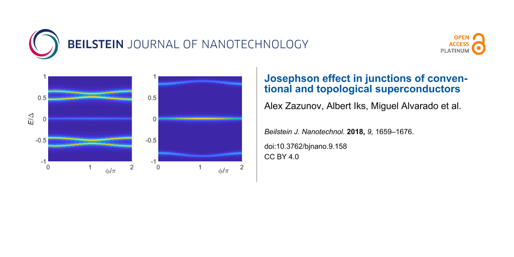
Phase dependence of the subgap spectrum of an S–QD–TS junction in the noninteracting case, U = 0. The TS wire is modeled from the low-energy limit of a Kitaev chain, and we use the parameters By = 0, Bx = Bz = B/![[Graphic 43]](/bjnano/content/inline/2190-4286-9-158-i105.svg?max-width=637&scale=1.18182) , ε0 = 0, Δp = Δ, and ΓS = ΓTS = Γ. From blue to yellow, the color code indicates increasing values of the spectral density. The left (right) panel is for Γ = 0.045Δ and B = 0.1Δ (Γ = B = 0.5Δ). Solid curves were obtained by numerical evaluation of Equation 30. Dashed curves give the analytical prediction (Equation 32). In the right panel, the energies resulting from Equation 32 have been rescaled by the factor 1 + Γ/Δ.
, ε0 = 0, Δp = Δ, and ΓS = ΓTS = Γ. From blue to yellow, the color code indicates increasing values of the spectral density. The left (right) panel is for Γ = 0.045Δ and B = 0.1Δ (Γ = B = 0.5Δ). Solid curves were obtained by numerical evaluation of Equation 30. Dashed curves give the analytical prediction (Equation 32). In the right panel, the energies resulting from Equation 32 have been rescaled by the factor 1 + Γ/Δ.
Figure 2: Phase dependence of the subgap spectrum of an S–QD–TS junction in the noninteracting case, U = 0. T...
We next turn to self-consistent mean-field results for the phase-dependent ABS spectrum at finite U. Figure 3 shows the spectrum for the electron–hole symmetric case ε0 = −U/2, with other parameters as in the right panel of Figure 2. For moderate interaction strength, e.g., taking U = Δ (left panel), we find that compared to the U = 0 case in Figure 2, interactions push together pairs of Andreev bands, e.g., the pair corresponding to ![[Graphic 44]](/bjnano/content/inline/2190-4286-9-158-i106.svg?max-width=637&scale=1.18182) in Equation 30. On the other hand, for stronger interactions, e.g., U = 10Δ (right panel), the outer ABSs leak into the continuum spectrum and only the inner Andreev states remain inside the superconducting gap. The ABS spectrum shown in Figure 3 is similar to what is observed in mean-field calculations for S–QD–S systems with broken spin symmetry and in the magnetic regime of the QD, where one finds up to four ABSs for U < Δ while the outer ABSs merge with the continuum for U > Δ [79]. Interestingly, the inner ABS contribution to the free energy for U = 10Δ is minimal for
in Equation 30. On the other hand, for stronger interactions, e.g., U = 10Δ (right panel), the outer ABSs leak into the continuum spectrum and only the inner Andreev states remain inside the superconducting gap. The ABS spectrum shown in Figure 3 is similar to what is observed in mean-field calculations for S–QD–S systems with broken spin symmetry and in the magnetic regime of the QD, where one finds up to four ABSs for U < Δ while the outer ABSs merge with the continuum for U > Δ [79]. Interestingly, the inner ABS contribution to the free energy for U = 10Δ is minimal for ![[Graphic 45]](/bjnano/content/inline/2190-4286-9-158-i107.svg?max-width=637&scale=1.18182) = π, see right panel of Figure 3, and we therefore expect π-junction behavior for By = 0 also in the regime with U
= π, see right panel of Figure 3, and we therefore expect π-junction behavior for By = 0 also in the regime with U ![[Graphic 46]](/bjnano/content/inline/2190-4286-9-158-i108.svg?max-width=637&scale=1.18182) Δ and B
Δ and B ![[Graphic 47]](/bjnano/content/inline/2190-4286-9-158-i109.svg?max-width=637&scale=1.18182) Δ. We notice, however, that changing the sign of Bx would result in zero junction behavior. We interpret the inner ABSs for U
Δ. We notice, however, that changing the sign of Bx would result in zero junction behavior. We interpret the inner ABSs for U ![[Graphic 48]](/bjnano/content/inline/2190-4286-9-158-i110.svg?max-width=637&scale=1.18182) Δ as Shiba states with the phase dependence generated by the coupling to the MBS. Without the latter coupling, the Shiba state has
Δ as Shiba states with the phase dependence generated by the coupling to the MBS. Without the latter coupling, the Shiba state has ![[Graphic 49]](/bjnano/content/inline/2190-4286-9-158-i111.svg?max-width=637&scale=1.18182) -independent energy slightly below Δ determined by the scattering phase shift difference between both spin polarizations [80].
-independent energy slightly below Δ determined by the scattering phase shift difference between both spin polarizations [80].
![[2190-4286-9-158-3]](/bjnano/content/figures/2190-4286-9-158-3.png?scale=2.0&max-width=1024&background=FFFFFF)
Figure 3:
Phase-dependent ABS spectrum from mean-field theory for S–QD–TS junctions as in Figure 2 but with U > 0 and ε0 = −U/2. We put Δp = Δ, By = 0, and ΓS = ΓTS = Γ. The color code is as in Figure 2. The left panel is for U = Δ, Γ = 0.5Δ, and Bx = Bz = B/![[Graphic 50]](/bjnano/content/inline/2190-4286-9-158-i112.svg?max-width=637&scale=1.18182) with B = 0.5Δ [cf. the right panel of Figure 2]. The right panel is for U = 10Δ, Γ = 4.5Δ, Bx = 15Δ, and Bz = 0.
with B = 0.5Δ [cf. the right panel of Figure 2]. The right panel is for U = 10Δ, Γ = 4.5Δ, Bx = 15Δ, and Bz = 0.
Figure 3: Phase-dependent ABS spectrum from mean-field theory for S–QD–TS junctions as in Figure 2 but with U > 0 and...
As illustrated in Figure 4, the CPR computed numerically from Equation 30 for different values of ΓS,TS/Δ, where Bx has been inverted with respect to its value in Figure 3, results in zero junction behavior. This behavior is expected from Equation 23 in the cotunneling regime, and Figure 4 shows that it also persists for ΓS,TS ![[Graphic 51]](/bjnano/content/inline/2190-4286-9-158-i113.svg?max-width=637&scale=1.18182) Δ. In contrast to Equation 23, however, the CPR for ΓS,TS
Δ. In contrast to Equation 23, however, the CPR for ΓS,TS ![[Graphic 52]](/bjnano/content/inline/2190-4286-9-158-i114.svg?max-width=637&scale=1.18182) Δ differs from a purely sinusoidal behavior, see Figure 4. Moreover, for By ≠ 0, we again encounter φ0-junction behavior, cf. the inset of Figure 4, in accordance with the perturbative result in Equation 23. Our mean-field results suggest that φ0-junction behavior is very robust and extends also into other parameter regimes as long as the condition By ≠ 0 is met.
Δ differs from a purely sinusoidal behavior, see Figure 4. Moreover, for By ≠ 0, we again encounter φ0-junction behavior, cf. the inset of Figure 4, in accordance with the perturbative result in Equation 23. Our mean-field results suggest that φ0-junction behavior is very robust and extends also into other parameter regimes as long as the condition By ≠ 0 is met.
![[2190-4286-9-158-4]](/bjnano/content/figures/2190-4286-9-158-4.png?scale=2.0&max-width=1024&background=FFFFFF)
Figure 4:
Main panel: Mean-field results for the CPR of S–QD–TS junctions with different Γ/Δ values, where we assume Δp = Δ, U = 10Δ, ε0 = −U/2, ΓS = ΓTS = Γ, B = 15Δ, and Bz = 0. Main panel: For Bx = −B and By = 0. Inset: Same but for By = −Bx = B/![[Graphic 53]](/bjnano/content/inline/2190-4286-9-158-i115.svg?max-width=637&scale=1.18182) , where φ0-junction behavior occurs.
, where φ0-junction behavior occurs.
Figure 4: Main panel: Mean-field results for the CPR of S–QD–TS junctions with different Γ/Δ values, where we...
Next, Figure 5 shows mean-field results for the critical current, ![[Graphic 54]](/bjnano/content/inline/2190-4286-9-158-i116.svg?max-width=637&scale=1.18182) |I(
|I(![[Graphic 55]](/bjnano/content/inline/2190-4286-9-158-i117.svg?max-width=637&scale=1.18182) )|, as function of the local magnetic field Bx and otherwise the same parameters as in Figure 4. The main panel in Figure 5 shows that Ic increases linearly with Bx for small Bx < Δ, then exhibits a maximum around Bx ≈ Γ, and subsequently decreases again to small values for Bx
)|, as function of the local magnetic field Bx and otherwise the same parameters as in Figure 4. The main panel in Figure 5 shows that Ic increases linearly with Bx for small Bx < Δ, then exhibits a maximum around Bx ≈ Γ, and subsequently decreases again to small values for Bx ![[Graphic 56]](/bjnano/content/inline/2190-4286-9-158-i118.svg?max-width=637&scale=1.18182) max{ΓS,TS,Δ}. On the other hand, for a fixed absolute value B of the magnetic field and By = 0, the critical current also exhibits a maximum as a function of the angle θB between B and the MBS spin polarization axis (
max{ΓS,TS,Δ}. On the other hand, for a fixed absolute value B of the magnetic field and By = 0, the critical current also exhibits a maximum as a function of the angle θB between B and the MBS spin polarization axis (![[Graphic 57]](/bjnano/content/inline/2190-4286-9-158-i119.svg?max-width=637&scale=1.18182) ). This effect is illustrated in the inset of Figure 5. As expected, the Josephson current vanishes for θB → 0, where the supercurrent blockade argument of [31] implies Ic = 0, and reaches its maximal value for θB = π/2.
). This effect is illustrated in the inset of Figure 5. As expected, the Josephson current vanishes for θB → 0, where the supercurrent blockade argument of [31] implies Ic = 0, and reaches its maximal value for θB = π/2.
![[2190-4286-9-158-5]](/bjnano/content/figures/2190-4286-9-158-5.png?scale=2.0&max-width=1024&background=FFFFFF)
Figure 5: Main panel: Mean-field results for the critical current Ic vs local magnetic field scale Bx in S–QD–TS junctions. Parameters are as in the main panel of Figure 4, i.e., U = 10Δ, ε0 = −U/2, and By,z = 0. From left to right, different curves are for Γ/Δ = 4.5, 8, 10 and 12.5. Inset: Ic vs angle θB, where B = B (sinθB,0,cosθB) with B = 15Δ.
Figure 5: Main panel: Mean-field results for the critical current Ic vs local magnetic field scale Bx in S–QD...
Spinful nanowire model for the TS
Model
Before turning to the S–TS–S setup in Figure 1b, we address the question of how the above results for S–QD–TS junctions change when using the spinful nanowire model of [2,3] instead of the low-energy limit of a Kitaev chain, see Equation 7. In fact, we will first describe the Josephson current for the elementary case of an S–TS junction using the spinful nanowire model. Surprisingly, to the best of our knowledge, this case has not yet been addressed in the literature.
In spatially discretized form, the spinful nanowire model for TS wires reads [2,3,43]
![[2190-4286-9-158-i34]](/bjnano/content/inline/2190-4286-9-158-i34.svg?max-width=590&scale=1.18182)
where the lattice fermion operators cjσ for given site j with spin polarizations σ = ↑,↓ are combined to the four-spinor operator
![[Graphic 58]](/bjnano/content/inline/2190-4286-9-158-i120.svg?max-width=637&scale=1.18182)
The Pauli matrices τx,y,z (and unity τ0) again act in Nambu space, while Pauli matrices σx,y,z and σ0 refer to spin. In the figures shown below, we choose the model parameters in Equation 34 as discussed in [43]. The lattice spacing is set to a = 10 nm, which results in a nearest-neighbor hopping t = ![[Graphic 59]](/bjnano/content/inline/2190-4286-9-158-i121.svg?max-width=637&scale=1.18182) 2/(2m*a2) = 20 meV and the spin–orbit coupling strength α = 4 meV for InAs nanowires. The proximity-induced pairing gap is again denoted by Δp, the chemical potential is μ, and the bulk Zeeman energy scale Vx is determined by a magnetic field applied along the wire. Under the condition
2/(2m*a2) = 20 meV and the spin–orbit coupling strength α = 4 meV for InAs nanowires. The proximity-induced pairing gap is again denoted by Δp, the chemical potential is μ, and the bulk Zeeman energy scale Vx is determined by a magnetic field applied along the wire. Under the condition
![[2190-4286-9-158-i35]](/bjnano/content/inline/2190-4286-9-158-i35.svg?max-width=590&scale=1.18182)
the topologically nontrivial phase is realized [2,3]. As we discuss below, the physics of the S–QD–TS junction sensitively depends on both the bulk Zeeman field Vx and on the local magnetic field B acting on the QD, where one can either identify both magnetic fields or treat B as independent field. In any case, the bGF ![[Graphic 60]](/bjnano/content/inline/2190-4286-9-158-i122.svg?max-width=637&scale=1.18182) (ω) for the model in Equation 34, which now replaces the Kitaev chain result G(ω) in Equation 7, needs to be computed numerically. The bGF
(ω) for the model in Equation 34, which now replaces the Kitaev chain result G(ω) in Equation 7, needs to be computed numerically. The bGF ![[Graphic 61]](/bjnano/content/inline/2190-4286-9-158-i123.svg?max-width=637&scale=1.18182) has been described in detail in [43], where also a straightforward numerical scheme for calculating
has been described in detail in [43], where also a straightforward numerical scheme for calculating ![[Graphic 62]](/bjnano/content/inline/2190-4286-9-158-i124.svg?max-width=637&scale=1.18182) (ω) has been devised. With the replacement G→
(ω) has been devised. With the replacement G→![[Graphic 63]](/bjnano/content/inline/2190-4286-9-158-i125.svg?max-width=637&scale=1.18182) , we can then take over the expressions for the Josephson current discussed before. Below we study these expressions in the zero-temperature limit.
, we can then take over the expressions for the Josephson current discussed before. Below we study these expressions in the zero-temperature limit.
S–TS junction
Let us first address the CPR for the S–TS junction case. The Josephson current can be computed using the bGF expression for tunnel junctions in [40], which is a simplified version of the above expressions for the S–QD–TS case. The spin-conserving tunnel coupling λ defines a transmission probability (transparency) ![[Graphic 64]](/bjnano/content/inline/2190-4286-9-158-i126.svg?max-width=637&scale=1.18182) of the normal junction [40,43]. Close to the topological transition, the transparency is well approximated by
of the normal junction [40,43]. Close to the topological transition, the transparency is well approximated by
![[2190-4286-9-158-i36]](/bjnano/content/inline/2190-4286-9-158-i36.svg?max-width=590&scale=1.18182)
where t = 20 meV is the hopping parameter in Equation 34. We then study the CPR and the resulting critical current Ic as a function of ![[Graphic 65]](/bjnano/content/inline/2190-4286-9-158-i127.svg?max-width=637&scale=1.18182) for both the topologically trivial (Vx <
for both the topologically trivial (Vx < ![[Graphic 66]](/bjnano/content/inline/2190-4286-9-158-i128.svg?max-width=637&scale=1.18182) ) and the nontrivial (Vx >
) and the nontrivial (Vx > ![[Graphic 67]](/bjnano/content/inline/2190-4286-9-158-i129.svg?max-width=637&scale=1.18182) ) regime, see Equation 35.
) regime, see Equation 35.
In Figure 6, we show the Vx dependence of the critical current Ic for the symmetric case Δ = Δp. In particular, it is of interest to determine how Ic changes as one moves through the phase transition in Equation 35. First, we observe that Ic is strongly suppressed in the topological phase in comparison to the topologically trivial phase. In fact, Ic slowly decreases as one moves into the deep topological phase by increasing Vx. This observation is in accordance with the expected supercurrent blockade in the deep topological limit [31]: Ic = 0 for the corresponding Kitaev chain case since p-wave pairing correlations on the TS side are incompatible with s-wave correlations on the S side. However, a residual finite supercurrent can be observed even for rather large values of Vx. We attribute this effect to the remaining s-wave pairing correlations contained in the spinful nanowire model (Equation 34). Second, Figure 6 shows kink-like features in the Ic(Vx) curve near the topological transition, Vx ≈ ![[Graphic 68]](/bjnano/content/inline/2190-4286-9-158-i130.svg?max-width=637&scale=1.18182) . The inset of Figure 6 demonstrates that this feature comes from a rapid decrease of the ABS contribution while the continuum contribution remains smooth. This observation suggests that continuum contributions in this setup mainly originate from s-wave pairing correlations which are not particularly sensitive to the topological transition.
. The inset of Figure 6 demonstrates that this feature comes from a rapid decrease of the ABS contribution while the continuum contribution remains smooth. This observation suggests that continuum contributions in this setup mainly originate from s-wave pairing correlations which are not particularly sensitive to the topological transition.
![[2190-4286-9-158-6]](/bjnano/content/figures/2190-4286-9-158-6.png?scale=2.0&max-width=1024&background=FFFFFF)
Figure 6:
Main panel: Critical current Ic vs Zeeman energy Vx for an S–TS junction using the spinful TS nanowire model (Equation 34) for Δp = Δ = 0.2 meV, μ = 5 meV, and different transparencies ![[Graphic 69]](/bjnano/content/inline/2190-4286-9-158-i131.svg?max-width=637&scale=1.18182) calculated from Equation 36. All other parameters are specified in the main text. Inset: Decomposition of Ic for
calculated from Equation 36. All other parameters are specified in the main text. Inset: Decomposition of Ic for ![[Graphic 70]](/bjnano/content/inline/2190-4286-9-158-i132.svg?max-width=637&scale=1.18182) = 1 into ABS (dotted-dashed) and continuum (dashed) contributions.
= 1 into ABS (dotted-dashed) and continuum (dashed) contributions.
Figure 6: Main panel: Critical current Ic vs Zeeman energy Vx for an S–TS junction using the spinful TS nanow...
In Figure 7, we show the CPR for the S–TS junction with ![[Graphic 71]](/bjnano/content/inline/2190-4286-9-158-i133.svg?max-width=637&scale=1.18182) = 1 in Figure 6, where different curves correspond to different Zeeman couplings Vx near the critical value. We find that in many parameter regions, in particular for
= 1 in Figure 6, where different curves correspond to different Zeeman couplings Vx near the critical value. We find that in many parameter regions, in particular for ![[Graphic 72]](/bjnano/content/inline/2190-4286-9-158-i134.svg?max-width=637&scale=1.18182) < 1, the CPR is to high accuracy given by a conventional 2π-periodic Josephson relation, I(
< 1, the CPR is to high accuracy given by a conventional 2π-periodic Josephson relation, I(![[Graphic 73]](/bjnano/content/inline/2190-4286-9-158-i135.svg?max-width=637&scale=1.18182) ) = Ic sin
) = Ic sin![[Graphic 74]](/bjnano/content/inline/2190-4286-9-158-i136.svg?max-width=637&scale=1.18182) . In the topologically trivial phase, small deviations from the sinusoidal law can be detected, but once one enters the topological phase, these deviations become extremely small.
. In the topologically trivial phase, small deviations from the sinusoidal law can be detected, but once one enters the topological phase, these deviations become extremely small.
![[2190-4286-9-158-7]](/bjnano/content/figures/2190-4286-9-158-7.png?scale=2.0&max-width=1024&background=FFFFFF)
Figure 7:
CPR for the S–TS junction with ![[Graphic 75]](/bjnano/content/inline/2190-4286-9-158-i137.svg?max-width=637&scale=1.18182) = 1 in Figure 6, for different bulk Zeeman fields Vx (in meV) near the critical value
= 1 in Figure 6, for different bulk Zeeman fields Vx (in meV) near the critical value ![[Graphic 76]](/bjnano/content/inline/2190-4286-9-158-i138.svg?max-width=637&scale=1.18182) = 5.004 meV.
= 5.004 meV.
Figure 7:
CPR for the S–TS junction with = 1 in Figure 6, for different bulk Zeeman fields Vx (in meV) near the crit...
S–QD–TS junction with spinful TS wire: Mean-field theory
Apart from providing a direct link to experimental control parameters, another advantage of using the spinful nanowire model of [2,3] for modeling the TS wire is that the angle between the local Zeeman field B and the MBS spin polarization does not have to be introduced as phenomenological parameter but instead results from the calculation [43]. It is thus interesting to study the Josephson current in S–QD–TS junctions where the TS wire is described by the spinful nanowire model. For this purpose, we now revisit the mean-field scheme for S–QD–TS junctions using the bGF ![[Graphic 77]](/bjnano/content/inline/2190-4286-9-158-i139.svg?max-width=637&scale=1.18182) (ω) for the spinful nanowire model (Equation 34). In particular, with the replacement G→
(ω) for the spinful nanowire model (Equation 34). In particular, with the replacement G→![[Graphic 78]](/bjnano/content/inline/2190-4286-9-158-i140.svg?max-width=637&scale=1.18182) , we solve the self-consistency equations (Equation 26) and thereby obtain the mean-field parameters in Equation 25. The resulting QD GF, Gd(ω) in Equation 27, then determines the Josephson current in Equation 30. Below we present self-consistent mean-field results obtained from this scheme. In view of the huge parameter space of this problem, we here only discuss a few key observations. A full discussion of the phase diagram and the corresponding physics will be given elsewhere.
, we solve the self-consistency equations (Equation 26) and thereby obtain the mean-field parameters in Equation 25. The resulting QD GF, Gd(ω) in Equation 27, then determines the Josephson current in Equation 30. Below we present self-consistent mean-field results obtained from this scheme. In view of the huge parameter space of this problem, we here only discuss a few key observations. A full discussion of the phase diagram and the corresponding physics will be given elsewhere.
The main panel of Figure 8 shows the critical current Ic vs the bulk Zeeman energy Vx for several values of the chemical potential μ, where the respective critical value ![[Graphic 79]](/bjnano/content/inline/2190-4286-9-158-i141.svg?max-width=637&scale=1.18182) in Equation 35 for the topological phase transition also changes with μ. The results in Figure 8 assume that the local magnetic field B acting on the QD coincides with the bulk Zeeman field Vx in the TS wire, i.e., B = (Vx,0,0). For the rather large values of ΓS,TS taken in Figure 8, the Ic vs Vx curves again exhibit a kink-like feature near the topological transition, Vx ≈
in Equation 35 for the topological phase transition also changes with μ. The results in Figure 8 assume that the local magnetic field B acting on the QD coincides with the bulk Zeeman field Vx in the TS wire, i.e., B = (Vx,0,0). For the rather large values of ΓS,TS taken in Figure 8, the Ic vs Vx curves again exhibit a kink-like feature near the topological transition, Vx ≈ ![[Graphic 80]](/bjnano/content/inline/2190-4286-9-158-i142.svg?max-width=637&scale=1.18182) . This behavior is very similar to what happens in S–TS junctions with large transparency
. This behavior is very similar to what happens in S–TS junctions with large transparency ![[Graphic 81]](/bjnano/content/inline/2190-4286-9-158-i143.svg?max-width=637&scale=1.18182) , cf. Figure 6. As demonstrated in the inset of Figure 8, the physical reason for the kink feature can be traced back to a sudden drop of the ABS contribution to Ic when entering the topological phase Vx >
, cf. Figure 6. As demonstrated in the inset of Figure 8, the physical reason for the kink feature can be traced back to a sudden drop of the ABS contribution to Ic when entering the topological phase Vx > ![[Graphic 82]](/bjnano/content/inline/2190-4286-9-158-i144.svg?max-width=637&scale=1.18182) . In the latter phase, Ic becomes strongly suppressed in close analogy to the S–TS junction case shown in Figure 6.
. In the latter phase, Ic becomes strongly suppressed in close analogy to the S–TS junction case shown in Figure 6.
![[2190-4286-9-158-8]](/bjnano/content/figures/2190-4286-9-158-8.png?scale=2.0&max-width=1024&background=FFFFFF)
Figure 8:
Main panel: Critical current Ic vs Zeeman energy Vx for S–QD–TS junctions from mean-field theory using the spinful TS nanowire model (Equation 34). Results are shown for several values of the chemical potential μ (in meV), where we assume U = 10Δ, ε0 = −U/2, Δp = Δ = 0.2 meV, ΓS = 2ΓTS = 9Δ, and B = (Vx,0,0). Inset: Detailed view of the transition region Vx ≈ ![[Graphic 83]](/bjnano/content/inline/2190-4286-9-158-i145.svg?max-width=637&scale=1.18182) for μ = 4 meV, including a decomposition of Ic into the ABS (dotted-dashed) and the continuum (dashed) contribution.
for μ = 4 meV, including a decomposition of Ic into the ABS (dotted-dashed) and the continuum (dashed) contribution.
Figure 8: Main panel: Critical current Ic vs Zeeman energy Vx for S–QD–TS junctions from mean-field theory us...
In Figure 8, both the QD and the TS wire were subject to the same magnetic Zeeman field. If the direction and/or the size of the local magnetic field B applied to the QD can be varied independently from the bulk magnetic field Vx![[Graphic 84]](/bjnano/content/inline/2190-4286-9-158-i146.svg?max-width=637&scale=1.18182) applied to the TS wire, one can arrive at rather different conclusions. To illustrate this statement, Figure 9 shows the Ic vs Bz dependence for B = (0,0,Bz) perpendicular to the bulk field, with Vx >
applied to the TS wire, one can arrive at rather different conclusions. To illustrate this statement, Figure 9 shows the Ic vs Bz dependence for B = (0,0,Bz) perpendicular to the bulk field, with Vx > ![[Graphic 85]](/bjnano/content/inline/2190-4286-9-158-i147.svg?max-width=637&scale=1.18182) such that the TS wire is in the topological phase. In this case, Figure 9 shows that Ic exhibits a maximum close to Bz ~ Γ. This behavior is reminiscent of what we observed above in Figure 5, using the low-energy limit of a Kitaev chain for the bGF of the TS wire. Remarkably, the critical current can here reach values close to the unitary limit, Ic ~ eΔ/
such that the TS wire is in the topological phase. In this case, Figure 9 shows that Ic exhibits a maximum close to Bz ~ Γ. This behavior is reminiscent of what we observed above in Figure 5, using the low-energy limit of a Kitaev chain for the bGF of the TS wire. Remarkably, the critical current can here reach values close to the unitary limit, Ic ~ eΔ/![[Graphic 86]](/bjnano/content/inline/2190-4286-9-158-i148.svg?max-width=637&scale=1.18182) . We note that since Bz does not drive a phase transition, no kink-like features appear for the Ic(Bz) curves shown in Figure 9. Finally, the inset of Figure 9 shows that for B perpendicular to Vx
. We note that since Bz does not drive a phase transition, no kink-like features appear for the Ic(Bz) curves shown in Figure 9. Finally, the inset of Figure 9 shows that for B perpendicular to Vx![[Graphic 87]](/bjnano/content/inline/2190-4286-9-158-i149.svg?max-width=637&scale=1.18182) , where Vx >
, where Vx > ![[Graphic 88]](/bjnano/content/inline/2190-4286-9-158-i150.svg?max-width=637&scale=1.18182) for the parameters chosen in Figure 9, the ABSs provide the dominant contribution to the current in this regime.
for the parameters chosen in Figure 9, the ABSs provide the dominant contribution to the current in this regime.
![[2190-4286-9-158-9]](/bjnano/content/figures/2190-4286-9-158-9.png?scale=2.0&max-width=1024&background=FFFFFF)
Figure 9:
Main panel: Mean-field results for Ic vs Bz in S–QD–TS junctions for several values of ΓS = ΓTS = Γ (in meV) and μ = 4 meV. The bulk Zeeman field Vx = 5 meV along ![[Graphic 89]](/bjnano/content/inline/2190-4286-9-158-i151.svg?max-width=637&scale=1.18182) (where Vx >
(where Vx > ![[Graphic 90]](/bjnano/content/inline/2190-4286-9-158-i152.svg?max-width=637&scale=1.18182) for our parameters) is applied to the spinful TS wire, while the QD is subject to the local magnetic field B = Bz
for our parameters) is applied to the spinful TS wire, while the QD is subject to the local magnetic field B = Bz![[Graphic 91]](/bjnano/content/inline/2190-4286-9-158-i153.svg?max-width=637&scale=1.18182) . All other parameters are as in Figure 8. Inset: Decomposition of Ic into ABS (dotted-dashed) and continuum (dashed) contributions for Γ = 1.6 meV.
. All other parameters are as in Figure 8. Inset: Decomposition of Ic into ABS (dotted-dashed) and continuum (dashed) contributions for Γ = 1.6 meV.
Figure 9: Main panel: Mean-field results for Ic vs Bz in S–QD–TS junctions for several values of ΓS = ΓTS = Γ...
S–TS–S junctions: Switching the parity of a superconducting atomic contact
Model
We now proceed to the three-terminal S–TS–S setup shown in Figure 1b. The CPR found in the related TS–S–TS trijunction case has been discussed in detail in [43], see also [44]. Among other findings, a main conclusion of [43] for the TS–S–TS geometry was that the CPR can reveal information about the spin canting angle between the MBS spin polarization axes in both TS wires. In what follows, we study the superficially similar yet rather different case of an S–TS–S junction. Throughout this section, we model the TS wire via the low-energy theory of a spinless Kitaev chain, where the bGF G(ω) in Equation 7 applies.
One can view the setup in Figure 1b as a conventional superconducting atomic contact (SAC) with a TS wire tunnel-coupled to the S–S junction. Over the past few years, impressive experimental progress [52-54] has demonstrated that the ABS level system in a SAC [81] can be accurately probed and manipulated by coherent or incoherent microwave spectroscopy techniques. We show below that an additional TS wire, cf. Figure 1b, acts as tunable parity switch on the many-body ABS levels of the SAC. As we have discussed above, the supercurrent flowing directly between a given S lead and the TS wire is expected to be strongly suppressed. However, through the hybridization with the MBS, Andreev level configurations with even and odd fermion parity are connected. This effect has profound and potentially useful consequences for Andreev spectroscopy.
An alternative view of the setup in Figure 1b is to imagine an S–TS junction, where S1 plays the role of the S lead and the spinful TS wire is effectively composed from a spinless (Kitaev) TS wire and the S2 superconductor. The p- and s-wave pairing correlations in the spinful TS wire are thereby spatially separated. Since the s- and p-wave bands represent normal modes, they are not directly coupled to each other in this scenario, i.e., we have to put λ2 = 0. We discuss this analogy in more detail later on.
We consider a conventional single-channel SAC (gap Δ) coupled via a point contact to a TS wire (gap Δp), cf. Figure 1b. The superconducting phase difference across the SAC is denoted by ![[Graphic 92]](/bjnano/content/inline/2190-4286-9-158-i154.svg?max-width=637&scale=1.18182) where
where ![[Graphic 93]](/bjnano/content/inline/2190-4286-9-158-i155.svg?max-width=637&scale=1.18182) is the phase difference between the respective S arm (j = 1,2) and the TS wire. In practice, the SAC can be embedded into a superconducting ring for magnetic flux tuning of
is the phase difference between the respective S arm (j = 1,2) and the TS wire. In practice, the SAC can be embedded into a superconducting ring for magnetic flux tuning of ![[Graphic 94]](/bjnano/content/inline/2190-4286-9-158-i156.svg?max-width=637&scale=1.18182) . To allow for analytical progress, we here assume that Δp is so large that continuum quasiparticle excitations in the TS wire can be neglected. In that case, only the MBS at the junction has to be kept when modeling the TS wire. However, we will also hint at how one can treat the general case.
. To allow for analytical progress, we here assume that Δp is so large that continuum quasiparticle excitations in the TS wire can be neglected. In that case, only the MBS at the junction has to be kept when modeling the TS wire. However, we will also hint at how one can treat the general case.
For the two S leads, boundary fermion fields are contained in Nambu spinors as in Equation 6,
![[2190-4286-9-158-i37]](/bjnano/content/inline/2190-4286-9-158-i37.svg?max-width=590&scale=1.18182)
where their bGF follows with the Nambu matrix g(ω) in Equation 6 as
![[2190-4286-9-158-i38]](/bjnano/content/inline/2190-4286-9-158-i38.svg?max-width=590&scale=1.18182)
We again use Pauli matrices τx,y,z and unity τ0 in Nambu space. The dimensionless parameters b1,2 describe the Zeeman field component along the MBS spin polarization axis, see below. Since above-gap quasiparticles in the TS wire are neglected here, the TS wire is represented by the Majorana operator γ = γ†, with γ2 = 1/2, which anticommutes with all other fermions. We may represent γ by an auxiliary fermion f↑, where the index reminds us that the MBS spin polarization points along ![[Graphic 95]](/bjnano/content/inline/2190-4286-9-158-i157.svg?max-width=637&scale=1.18182) ,
,
![[2190-4286-9-158-i39]](/bjnano/content/inline/2190-4286-9-158-i39.svg?max-width=590&scale=1.18182)
The other Majorana mode γ′ = ![[Graphic 96]](/bjnano/content/inline/2190-4286-9-158-i158.svg?max-width=637&scale=1.18182) which is localized at the opposite end of the TS wire, is assumed to have negligible hybridization with the ΨS,j spinors and with γ. Writing the Euclidean action as S = S0 + Stun, we have an uncoupled action contribution,
which is localized at the opposite end of the TS wire, is assumed to have negligible hybridization with the ΨS,j spinors and with γ. Writing the Euclidean action as S = S0 + Stun, we have an uncoupled action contribution,
![[2190-4286-9-158-i40]](/bjnano/content/inline/2190-4286-9-158-i40.svg?max-width=590&scale=1.18182)
The leads are connected by a time-local tunnel action corresponding to the tunnel Hamiltonian
![[2190-4286-9-158-i41]](/bjnano/content/inline/2190-4286-9-158-i41.svg?max-width=590&scale=1.18182)
Without loss of generality, we assume that the tunnel amplitudes t0 and λ1,2, see Figure 1b, are real-valued and that they include density-of-state factors again. The parameter t0 (with 0 ≤ t0 ≤ 1) determines the transparency ![[Graphic 97]](/bjnano/content/inline/2190-4286-9-158-i159.svg?max-width=637&scale=1.18182) of the SAC in the normal-conducting state [36], cf. Equation 36,
of the SAC in the normal-conducting state [36], cf. Equation 36,
![[2190-4286-9-158-i42]](/bjnano/content/inline/2190-4286-9-158-i42.svg?max-width=590&scale=1.18182)
Note that in Equation 41 we have again assumed spin-conserving tunneling, where only spin-↑ fermions in the SAC are tunnel-coupled to the Majorana fermion γ, cf. Equation 4.
At this stage, it is convenient to trace out the ΨS,2 spinor field. As a result, the SAC is described in terms of only one spinor field, Ψ ≡ ΨS,1, which however is still coupled to the Majorana field γ. After some algebra, we obtain the effective action
![[2190-4286-9-158-i43]](/bjnano/content/inline/2190-4286-9-158-i43.svg?max-width=590&scale=1.18182)
where the operator P↑ = (τ0 + τz)/2 projects a Nambu spinor to its spin-↑ component. Moreover, we have defined an effective GF in Nambu space with frequency components
![[2190-4286-9-158-i44]](/bjnano/content/inline/2190-4286-9-158-i44.svg?max-width=590&scale=1.18182)
and the TS lead has been represented by the Majorana–Nambu spinor
![[2190-4286-9-158-i45]](/bjnano/content/inline/2190-4286-9-158-i45.svg?max-width=590&scale=1.18182)
We note in passing that Equation 43 could at this point be generalized to include continuum states in the TS wire. To that end, one has to (i) replace Φ → (ψ, ψ†)T, where ψ is the boundary fermion of the effectively spinless TS wire, and (ii) replace δ(τ − τ′)∂τ′ → G−1(τ − τ′) with G in Equation 7. Including bulk TS quasiparticles becomes necessary for small values of the proximity gap, Δp ![[Graphic 98]](/bjnano/content/inline/2190-4286-9-158-i160.svg?max-width=637&scale=1.18182) Δ, and/or when studying nonequilibrium applications within a Keldysh version of our formalism.
Δ, and/or when studying nonequilibrium applications within a Keldysh version of our formalism.
In any case, after neglecting the above-gap TS continuum quasiparticles, the partition function follows with Seff in Equation 43 in the functional integral representation
![[2190-4286-9-158-i46]](/bjnano/content/inline/2190-4286-9-158-i46.svg?max-width=590&scale=1.18182)
As before, the Josephson current through S lead no. j then follows from the free energy via
![[Graphic 99]](/bjnano/content/inline/2190-4286-9-158-i161.svg?max-width=637&scale=1.18182)
The supercurrent flowing through the TS wire is then given by
![[2190-4286-9-158-i47]](/bjnano/content/inline/2190-4286-9-158-i47.svg?max-width=590&scale=1.18182)
as dictated by current conservation.
Atomic limit
In order to get insight into the basic physics, we now analyze in detail the atomic limit, where Δ represents the largest energy scale of interest and hence the dynamics is confined to the subgap region. In this case, we can approximate ![[Graphic 100]](/bjnano/content/inline/2190-4286-9-158-i162.svg?max-width=637&scale=1.18182) . After the rescaling
. After the rescaling
![[Graphic 101]](/bjnano/content/inline/2190-4286-9-158-i163.svg?max-width=637&scale=1.18182)
in Equation 43, we arrive at an effective action, Seff → Sat, valid in the atomic limit,
![[2190-4286-9-158-i48]](/bjnano/content/inline/2190-4286-9-158-i48.svg?max-width=590&scale=1.18182)
where ![[Graphic 102]](/bjnano/content/inline/2190-4286-9-158-i164.svg?max-width=637&scale=1.18182) is the reflection amplitude of the SAC, see Equation 42. We recall that
is the reflection amplitude of the SAC, see Equation 42. We recall that ![[Graphic 103]](/bjnano/content/inline/2190-4286-9-158-i165.svg?max-width=637&scale=1.18182) , see Equation 37. Moreover, we define the auxiliary parameters
, see Equation 37. Moreover, we define the auxiliary parameters
![[2190-4286-9-158-i49]](/bjnano/content/inline/2190-4286-9-158-i49.svg?max-width=590&scale=1.18182)
The parameters b1,2 in Equation 38 thus effectively generate the Zeeman scale Bz in Equation 49.
As a consequence of the atomic limit approximation, the action Sat in Equation 48 is equivalently expressed in terms of the effective Hamiltonian
![[2190-4286-9-158-i50]](/bjnano/content/inline/2190-4286-9-158-i50.svg?max-width=590&scale=1.18182)
where we define
![[2190-4286-9-158-i51]](/bjnano/content/inline/2190-4286-9-158-i51.svg?max-width=590&scale=1.18182)
For a SAC decoupled from the TS wire and taken at zero field (Bz = 0), the ABS energy follows from Equation 50 in the standard form [62]
![[2190-4286-9-158-i52]](/bjnano/content/inline/2190-4286-9-158-i52.svg?max-width=590&scale=1.18182)
We emphasize that Hat neglects TS continuum quasiparticles as well as all types of quasiparticle poisoning processes. Let us briefly pause in order to make two remarks. First, we note that the Majorana field
![[Graphic 104]](/bjnano/content/inline/2190-4286-9-158-i166.svg?max-width=637&scale=1.18182)
see Equation 39, couples to both spin modes ψσ in Equation 50. The coupling λ↓ between γ and the spin-↓ field in the SAC, ψ↓, is generated by crossed Andreev reflection processes, where a Cooper pair in lead S2 splits according to ![[Graphic 105]](/bjnano/content/inline/2190-4286-9-158-i167.svg?max-width=637&scale=1.18182) , plus the conjugate process. Second, we observe that Hat is invariant under a particle–hole transformation, amounting to the replacements
, plus the conjugate process. Second, we observe that Hat is invariant under a particle–hole transformation, amounting to the replacements ![[Graphic 106]](/bjnano/content/inline/2190-4286-9-158-i168.svg?max-width=637&scale=1.18182) and
and ![[Graphic 107]](/bjnano/content/inline/2190-4286-9-158-i169.svg?max-width=637&scale=1.18182) , along with Bz → − Bz and
, along with Bz → − Bz and ![[Graphic 108]](/bjnano/content/inline/2190-4286-9-158-i170.svg?max-width=637&scale=1.18182) → 2π −
→ 2π − ![[Graphic 109]](/bjnano/content/inline/2190-4286-9-158-i171.svg?max-width=637&scale=1.18182) .
.
We next notice that with nσ = ![[Graphic 110]](/bjnano/content/inline/2190-4286-9-158-i172.svg?max-width=637&scale=1.18182) = 0,1 and nf =
= 0,1 and nf = ![[Graphic 111]](/bjnano/content/inline/2190-4286-9-158-i173.svg?max-width=637&scale=1.18182) = 0,1, the total fermion parity of the junction,
= 0,1, the total fermion parity of the junction,
![[2190-4286-9-158-i53]](/bjnano/content/inline/2190-4286-9-158-i53.svg?max-width=590&scale=1.18182)
is a conserved quantity, [![[Graphic 112]](/bjnano/content/inline/2190-4286-9-158-i174.svg?max-width=637&scale=1.18182) , Hat]− = 0. Below we restrict our analysis to the even-parity sector
, Hat]− = 0. Below we restrict our analysis to the even-parity sector ![[Graphic 113]](/bjnano/content/inline/2190-4286-9-158-i175.svg?max-width=637&scale=1.18182) = +1, but analogous results hold for the odd-parity case. The corresponding Hilbert subspace is spanned by four states,
= +1, but analogous results hold for the odd-parity case. The corresponding Hilbert subspace is spanned by four states,
![[2190-4286-9-158-i54]](/bjnano/content/inline/2190-4286-9-158-i54.svg?max-width=590&scale=1.18182)
where (n↑, n↓, nf) ![[Graphic 114]](/bjnano/content/inline/2190-4286-9-158-i176.svg?max-width=637&scale=1.18182) {(0,0,0), (1,1,0), (1,0,1), (0,1,1)} and
{(0,0,0), (1,1,0), (1,0,1), (0,1,1)} and ![[Graphic 115]](/bjnano/content/inline/2190-4286-9-158-i177.svg?max-width=637&scale=1.18182) is the vacuum state. In this basis, the Hamiltonian (Equation 50) has the matrix representation
is the vacuum state. In this basis, the Hamiltonian (Equation 50) has the matrix representation
![[2190-4286-9-158-i55]](/bjnano/content/inline/2190-4286-9-158-i55.svg?max-width=590&scale=1.18182)
The even-parity ground state energy, ![[Graphic 116]](/bjnano/content/inline/2190-4286-9-158-i178.svg?max-width=637&scale=1.18182) = min(ε), follows as the smallest root of the quartic equation
= min(ε), follows as the smallest root of the quartic equation
![[2190-4286-9-158-i56]](/bjnano/content/inline/2190-4286-9-158-i56.svg?max-width=590&scale=1.18182)
In order to obtain simple results, let us now consider the special case λ2 = 0, where the TS wire is directly coupled to lead S1 only, see Figure 1b. In that case, we also have λ↓= 0, see Equation 49, and Equation 56 implies the four eigenenergies ±ε± with
![[2190-4286-9-158-i57]](/bjnano/content/inline/2190-4286-9-158-i57.svg?max-width=590&scale=1.18182)
with ![[Graphic 117]](/bjnano/content/inline/2190-4286-9-158-i179.svg?max-width=637&scale=1.18182) , see Equation 49. The ground-state energy is thus given by
, see Equation 49. The ground-state energy is thus given by ![[Graphic 118]](/bjnano/content/inline/2190-4286-9-158-i180.svg?max-width=637&scale=1.18182) = −ε+. Since EG depends on the phases
= −ε+. Since EG depends on the phases ![[Graphic 119]](/bjnano/content/inline/2190-4286-9-158-i181.svg?max-width=637&scale=1.18182) only via the Andreev level energy EA(
only via the Andreev level energy EA(![[Graphic 120]](/bjnano/content/inline/2190-4286-9-158-i182.svg?max-width=637&scale=1.18182) ) in Equation 52, the Josephson current through the SAC is given by
) in Equation 52, the Josephson current through the SAC is given by
![[2190-4286-9-158-i58]](/bjnano/content/inline/2190-4286-9-158-i58.svg?max-width=590&scale=1.18182)
Note that Equation 47 then implies that no supercurrent flows into the TS wire.
Next we observe that in the absence of the TS probe (λ1 = 0), the even and odd fermion parity sectors of the SAC, ![[Graphic 121]](/bjnano/content/inline/2190-4286-9-158-i183.svg?max-width=637&scale=1.18182) , are decoupled, see Equation 55, and Equation 57 yields
, are decoupled, see Equation 55, and Equation 57 yields ![[Graphic 122]](/bjnano/content/inline/2190-4286-9-158-i184.svg?max-width=637&scale=1.18182) = −max(EA, |Bz|). Importantly, the Josephson current is therefore fully blocked if the ground state is in the
= −max(EA, |Bz|). Importantly, the Josephson current is therefore fully blocked if the ground state is in the ![[Graphic 123]](/bjnano/content/inline/2190-4286-9-158-i185.svg?max-width=637&scale=1.18182) = −1 sector, i.e., for |Bz| > EA(
= −1 sector, i.e., for |Bz| > EA(![[Graphic 124]](/bjnano/content/inline/2190-4286-9-158-i186.svg?max-width=637&scale=1.18182) ). For λ1 ≠ 0, however,
). For λ1 ≠ 0, however, ![[Graphic 125]](/bjnano/content/inline/2190-4286-9-158-i187.svg?max-width=637&scale=1.18182) is not conserved anymore. This implies that the MBS can act as parity switch between the two Andreev sectors with parity
is not conserved anymore. This implies that the MBS can act as parity switch between the two Andreev sectors with parity ![[Graphic 126]](/bjnano/content/inline/2190-4286-9-158-i188.svg?max-width=637&scale=1.18182) = ±1. Near the level crossing point at EA ≈ |Bz|, i.e., assuming
= ±1. Near the level crossing point at EA ≈ |Bz|, i.e., assuming ![[Graphic 127]](/bjnano/content/inline/2190-4286-9-158-i189.svg?max-width=637&scale=1.18182) we obtain
we obtain
![[2190-4286-9-158-i59]](/bjnano/content/inline/2190-4286-9-158-i59.svg?max-width=590&scale=1.18182)
which implies a nonvanishing supercurrent through the SAC even in the field-dominated regime, |Bz| > EA. The MBS therefore acts as a parity switch and leaves a trace in the CPR by lifting the supercurrent blockade.
Another interpretation
Interestingly, for λ2 = ![[Graphic 128]](/bjnano/content/inline/2190-4286-9-158-i190.svg?max-width=637&scale=1.18182) = 0, the S–TS–S setup in Figure 1b could also be viewed as a toy model for an S–TS junction, where the TS part corresponds to a spinful model. In that analogy, the Nambu spinor ΨS,1 stands for the S lead while the spinful TS wire is represented by (i) the Nambu spinor ΨS,2 which is responsible for the residual s-wave pairing correlations, and (ii) by the MF γ (or, more generally, by the Kitaev-chain spinless boundary fermion ψ) which encodes p-wave pairing correlations. Moreover, t0 and λ1 should now be understood as spin-conserving phenomenological tunnel couplings acting in the s–s and s–p wave channels, respectively. The phase difference across this effective S–TS junction is
= 0, the S–TS–S setup in Figure 1b could also be viewed as a toy model for an S–TS junction, where the TS part corresponds to a spinful model. In that analogy, the Nambu spinor ΨS,1 stands for the S lead while the spinful TS wire is represented by (i) the Nambu spinor ΨS,2 which is responsible for the residual s-wave pairing correlations, and (ii) by the MF γ (or, more generally, by the Kitaev-chain spinless boundary fermion ψ) which encodes p-wave pairing correlations. Moreover, t0 and λ1 should now be understood as spin-conserving phenomenological tunnel couplings acting in the s–s and s–p wave channels, respectively. The phase difference across this effective S–TS junction is ![[Graphic 129]](/bjnano/content/inline/2190-4286-9-158-i191.svg?max-width=637&scale=1.18182) =
= ![[Graphic 130]](/bjnano/content/inline/2190-4286-9-158-i192.svg?max-width=637&scale=1.18182) and the net S–TS tunnel coupling is given by
and the net S–TS tunnel coupling is given by ![[Graphic 131]](/bjnano/content/inline/2190-4286-9-158-i193.svg?max-width=637&scale=1.18182) . Putting λ1 = 0 in the topologically trivial phase of the TS wire, the Josephson current carried by Andreev states in the s–s channel is blocked when the ground state is in the odd parity sector of the SAC. For λ1 ≠ 0, the MBS-mediated switching between odd and even parity sectors will now be activated and thereby lift the supercurrent blockade.
. Putting λ1 = 0 in the topologically trivial phase of the TS wire, the Josephson current carried by Andreev states in the s–s channel is blocked when the ground state is in the odd parity sector of the SAC. For λ1 ≠ 0, the MBS-mediated switching between odd and even parity sectors will now be activated and thereby lift the supercurrent blockade.
Conventional midgap level
A similar behavior as predicted above for the MBS-induced parity switch between ![[Graphic 132]](/bjnano/content/inline/2190-4286-9-158-i194.svg?max-width=637&scale=1.18182) = ±1 sectors could also be expected from a conventional fermionic subgap state tunnel-coupled to the SAC. Such a subgap state may be represented, e.g., by a single-level quantum dot in the Coulomb blockade regime. In particular, for a midgap (zero-energy) level with the fermion operator d, the Hamiltonian Hat in Equation 50 has to be replaced with
= ±1 sectors could also be expected from a conventional fermionic subgap state tunnel-coupled to the SAC. Such a subgap state may be represented, e.g., by a single-level quantum dot in the Coulomb blockade regime. In particular, for a midgap (zero-energy) level with the fermion operator d, the Hamiltonian Hat in Equation 50 has to be replaced with
![[2190-4286-9-158-i60]](/bjnano/content/inline/2190-4286-9-158-i60.svg?max-width=590&scale=1.18182)
In the even total parity basis (Equation 54), the matrix representation of the Hamiltonian is then instead of Equation 55 given by
![[2190-4286-9-158-i61]](/bjnano/content/inline/2190-4286-9-158-i61.svg?max-width=590&scale=1.18182)
Assuming |λ↑| = |λ↓| ≡ λ, Equation 56 then yields the eigenenergies ±ε± with
![[2190-4286-9-158-i62]](/bjnano/content/inline/2190-4286-9-158-i62.svg?max-width=590&scale=1.18182)
Remarkably, the ABS spectra in Equation 62 and Equation 57 are rather similar for ![[Graphic 133]](/bjnano/content/inline/2190-4286-9-158-i195.svg?max-width=637&scale=1.18182) . However, the MBS will automatically be located at zero energy and thus represents a generic situation.
. However, the MBS will automatically be located at zero energy and thus represents a generic situation.
Conclusion
We close this paper by summarizing our main findings. We have studied the Josephson effect in different setups involving both conventional s-wave BCS superconductors (S leads) and topologically nontrivial 1D p-wave superconductors (TS leads) with Majorana end states. The TS wires have been described either by a spinless theory applicable in the deep topological regime, which has the advantage of allowing for analytical progress but makes it difficult to establish contact to experimental control parameters, or by a spinful nanowire model as suggested in [2,3]. We have employed a unified imaginary-time Green’s function approach to analyze the equilibrium properties of such devices, but a Keldysh generalization is straightforward and allows one to study also nonequilibrium applications.
For S–TS tunnel junctions, we find that in the topological phase of the TS wire, the supercurrent is mainly carried by above-gap continuum contributions. We confirm the expected supercurrent blockade [31] in the deep topological regime (where the spinless theory is fully valid and thus no residual s-wave pairing exists), while for realistic parameters, a small but finite critical current is found. To good approximation, the Josephson current obeys the usual 2π-periodic sinusoidal current–phase relation. The dependence of the critical current on the bulk Zeeman field driving the TS wire through the topological phase transition shows a kink-like feature at the critical value, which is caused by a sudden drop of the Andreev state contribution.
The supercurrent blockade in the deep topological phase could be lifted by adding a magnetic impurity to the junction, also allowing for the presence of a local magnetic field B. Such a magnetic impurity arises from a spin-degenerate quantum dot (QD), and we have studied the corresponding S–QD–TS problem for both the spinless and the spinful TS wire model. Based on analytical results valid in the cotunneling regime as well as numerical results within the mean-field approximation, we predict φ0-junction behavior (anomalous Josephson effect) for the current–phase relation when the TS wire is in the topological phase.
As a final example for devices combining conventional and topological superconductors, we have shown that S–TS–S devices allow for a Majorana-induced parity switch between Andreev state sectors with different parity in a superconducting atomic contact. This observation could be useful for future microwave spectroscopy experiments of Andreev qubits in such contacts.
References
-
Kitaev, A. Yu. Phys.-Usp. 2001, 44, 131. doi:10.1070/1063-7869/44/10S/S29
Return to citation in text: [1] [2] -
Lutchyn, R. M.; Sau, J. D.; Das Sarma, S. Phys. Rev. Lett. 2010, 105, 077001. doi:10.1103/physrevlett.105.077001
Return to citation in text: [1] [2] [3] [4] [5] [6] [7] [8] [9] [10] -
Oreg, Y.; Refael, G.; von Oppen, F. Phys. Rev. Lett. 2010, 105, 177002. doi:10.1103/physrevlett.105.177002
Return to citation in text: [1] [2] [3] [4] [5] [6] [7] [8] [9] [10] -
Alicea, J.; Oreg, Y.; Refael, G.; von Oppen, F.; Fisher, M. P. A. Nat. Phys. 2011, 7, 412. doi:10.1038/nphys1915
Return to citation in text: [1] -
Alicea, J. Rep. Prog. Phys. 2012, 75, 076501. doi:10.1088/0034-4885/75/7/076501
Return to citation in text: [1] [2] -
Leijnse, M.; Flensberg, K. Semicond. Sci. Technol. 2012, 27, 124003. doi:10.1088/0268-1242/27/12/124003
Return to citation in text: [1] -
Beenakker, C. W. J. Annu. Rev. Condens. Matter Phys. 2013, 4, 113. doi:10.1146/annurev-conmatphys-030212-184337
Return to citation in text: [1] -
Aasen, D.; Hell, M.; Mishmash, R. V.; Higginbotham, A.; Danon, J.; Leijnse, M.; Jespersen, T. S.; Folk, J. A.; Marcus, C. M.; Flensberg, K.; Alicea, J. Phys. Rev. X 2016, 6, 031016. doi:10.1103/physrevx.6.031016
Return to citation in text: [1] -
Landau, L. A.; Plugge, S.; Sela, E.; Altland, A.; Albrecht, S. M.; Egger, R. Phys. Rev. Lett. 2016, 116, 050501. doi:10.1103/physrevlett.116.050501
Return to citation in text: [1] -
Plugge, S.; Landau, L. A.; Sela, E.; Altland, A.; Flensberg, K.; Egger, R. Phys. Rev. B 2016, 94, 174514. doi:10.1103/physrevb.94.174514
Return to citation in text: [1] -
Plugge, S.; Rasmussen, A.; Egger, R.; Flensberg, K. New J. Phys. 2017, 19, 012001. doi:10.1088/1367-2630/aa54e1
Return to citation in text: [1] -
Aguado, R. Riv. Nuovo Cimento Soc. Ital. Fis. 2017, 40, 523. doi:10.1393/ncr/i2017-10141-9
Return to citation in text: [1] [2] -
Mourik, V.; Zuo, K.; Frolov, S. M.; Plissard, S. R.; Bakkers, E. P. A. M.; Kouwenhoven, L. P. Science 2012, 336, 1003. doi:10.1126/science.1222360
Return to citation in text: [1] -
Das, A.; Ronen, Y.; Most, Y.; Oreg, Y.; Heiblum, M.; Shtrikman, H. Nat. Phys. 2012, 8, 887. doi:10.1038/nphys2479
Return to citation in text: [1] -
Albrecht, S. M.; Higginbotham, A. P.; Madsen, M.; Kuemmeth, F.; Jespersen, T. S.; Nygård, J.; Krogstrup, P.; Marcus, C. M. Nature 2016, 531, 206. doi:10.1038/nature17162
Return to citation in text: [1] -
Deng, M. T.; Vaitiekenas, S.; Hansen, E. B.; Danon, J.; Leijnse, M.; Flensberg, K.; Nygård, J.; Krogstrup, P.; Marcus, C. M. Science 2016, 354, 1557. doi:10.1126/science.aaf3961
Return to citation in text: [1] [2] -
Gül, Ö.; Zhang, H.; de Vries, F. K.; van Veen, J.; Zuo, K.; Mourik, V.; Conesa-Boj, S.; Nowak, M. P.; van Woerkom, D. J.; Quintero-Pérez, M.; Cassidy, M. C.; Geresdi, A.; Koelling, S.; Car, D.; Plissard, S. R.; Bakkers, E. P. A. M.; Kouwenhoven, L. P. Nano Lett. 2017, 17, 2690. doi:10.1021/acs.nanolett.7b00540
Return to citation in text: [1] -
Albrecht, S. M.; Hansen, E. B.; Higginbotham, A. P.; Kuemmeth, F.; Jespersen, T. S.; Nygård, J.; Krogstrup, P.; Danon, J.; Flensberg, K.; Marcus, C. M. Phys. Rev. Lett. 2017, 118, 137701. doi:10.1103/physrevlett.118.137701
Return to citation in text: [1] -
Zhang, H.; Gül, Ö.; Conesa-Boj, S.; Nowak, M. P.; Wimmer, M.; Zuo, K.; Mourik, V.; de Vries, F. K.; van Veen, J.; de Moor, M. W. A.; Bommer, J. D. S.; van Woerkom, D.; Car, D.; Plissard, S. R.; Bakkers, E. P. A. M.; Quintero-Pérez, M.; Cassidy, M. C.; Koelling, S.; Goswami, S.; Watanabe, K.; Taniguchi, T.; Kouwenhoven, L. P. Nat. Commun. 2017, 8, 16025. doi:10.1038/ncomms16025
Return to citation in text: [1] -
Nichele, F.; Drachmann, A. C. C.; Whiticar, A. M.; O’Farrell, E. C. T.; Suominen, H. J.; Fornieri, A.; Wang, T.; Gardner, G. C.; Thomas, C.; Hatke, A. T.; Krogstrup, P.; Manfra, M. J.; Flensberg, K.; Marcus, C. M. Phys. Rev. Lett. 2017, 119, 136803. doi:10.1103/physrevlett.119.136803
Return to citation in text: [1] -
Suominen, H. J.; Kjaergaard, M.; Hamilton, A. R.; Shabani, J.; Palmstrøm, C. J.; Marcus, C. M.; Nichele, F. Phys. Rev. Lett. 2017, 119, 176805. doi:10.1103/physrevlett.119.176805
Return to citation in text: [1] -
Gazibegovich, S.; Car, D.; Zhang, H.; Balk, S. C.; Logan, J. A.; de Moor, M. W. A.; Cassidy, M. C.; Schmits, R.; Xu, D.; Wang, G.; Krogstrup, P.; Op het Veld, R. L. M.; Shen, J.; Bouman, D.; Shojaei, B.; Pennachio, D.; Lee, J. S.; van Veldhoven, P. J.; Koelling, S.; Verheijen, M. A.; Kouwenhoven, L. P.; Palmstrøm, C. J.; Bakkers, E. P. A. M. Nature 2017, 548, 434. doi:10.1038/nature23468
Return to citation in text: [1] -
Zhang, H.; Liu, C.-X.; Gazibegovic, S.; Xu, D.; Logan, J. A.; Wang, G.; van Loo, N.; Bommer, J. D. S.; de Moor, M. W. A.; Car, D.; Op het Veld, R. L. M.; van Veldhoven, P. J.; Koelling, S.; Verheijen, M. A.; Pendharkar, M.; Pennachio, D. J.; Shojaei, B.; Lee, J. S.; Palmstrom, C. J.; Bakkers, E. P. A. M.; Das Sarma, S.; Kouwenhoven, L. P. Nature 2018, 556, 74–79. doi:10.1038/nature26142
Return to citation in text: [1] -
Deng, M. T.; Vaitiekénas, S.; Prada, E.; San-José, P.; Nygård, J.; Krogstrup, P.; Aguado, R.; Marcus, C. M. arXiv 2017, No. 1712.03536.
Return to citation in text: [1] -
Laroche, D.; Bouman, D.; van Woerkom, D. J.; Proutski, A.; Murthy, C.; Pikulin, D. I.; Nayak, C.; van Gulik, R. J. J.; Nygård, J.; Krogstrup, P.; Kouwenhoven, L. P.; Geresdi, A. arXiv 2017, No. 1712.08459.
Return to citation in text: [1] -
Nadj-Perge, S.; Drozdov, I. K.; Li, J.; Chen, H.; Jeon, S.; Seo, J.; MacDonald, A. H.; Bernevig, B. A.; Yazdani, A. Science 2014, 346, 602. doi:10.1126/science.1259327
Return to citation in text: [1] -
Ruby, M.; Pientka, F.; Peng, Y.; von Oppen, F.; Heinrich, B. W.; Franke, K. J. Phys. Rev. Lett. 2015, 115, 197204. doi:10.1103/physrevlett.115.197204
Return to citation in text: [1] -
Sun, H.-H.; Zhang, K.-W.; Hu, L.-H.; Li, C.; Wang, G.-Y.; Ma, H.-Y.; Xu, Z.-A.; Gao, C.-L.; Guan, D.-D.; Li, Y.-Y.; Liu, C.; Qian, D.; Zhou, Y.; Fu, L.; Li, S.-C.; Zhang, F.-C.; Jia, J.-F. Phys. Rev. Lett. 2016, 116, 257003. doi:10.1103/physrevlett.116.257003
Return to citation in text: [1] -
Feldman, B. E.; Randeria, M. T.; Li, J.; Jeon, S.; Xie, Y.; Wang, Z.; Drozdov, I. K.; Andrei Bernevig, B.; Yazdani, A. Nat. Phys. 2017, 13, 286. doi:10.1038/nphys3947
Return to citation in text: [1] -
Deacon, R. S.; Wiedenmann, J.; Bocquillon, E.; Domínguez, F.; Klapwijk, T. M.; Leubner, P.; Brüne, C.; Hankiewicz, E. M.; Tarucha, S.; Ishibashi, K.; Buhmann, H.; Molenkamp, L. W. Phys. Rev. X 2017, 7, 021011. doi:10.1103/physrevx.7.021011
Return to citation in text: [1] -
Zazunov, A.; Egger, R. Phys. Rev. B 2012, 85, 104514. doi:10.1103/physrevb.85.104514
Return to citation in text: [1] [2] [3] [4] [5] [6] -
Kwon, H.-J.; Sengupta, K.; Yakovenko, V. M. Eur. Phys. J. B 2004, 37, 349. doi:10.1140/epjb/e2004-00066-4
Return to citation in text: [1] -
Bratus, E. N.; Shumeiko, V. S.; Wendin, G. Phys. Rev. Lett. 1995, 74, 2110. doi:10.1103/physrevlett.74.2110
Return to citation in text: [1] -
Averin, D.; Bardas, A. Phys. Rev. Lett. 1995, 75, 1831. doi:10.1103/physrevlett.75.1831
Return to citation in text: [1] -
Cuevas, J. C.; Martín-Rodero, A.; Levy Yeyati, A. Phys. Rev. B 1996, 54, 7366. doi:10.1103/physrevb.54.7366
Return to citation in text: [1] -
Nazarov, Y.; Blanter, Y. Quantum Transport: Introduction to Nanoscience; Cambridge University Press: Cambridge, United Kingdom, 2010.
Return to citation in text: [1] [2] [3] [4] -
Peng, Y.; Pientka, F.; Vinkler-Aviv, Y.; Glazman, L. I.; von Oppen, F. Phys. Rev. Lett. 2015, 115, 266804. doi:10.1103/physrevlett.115.266804
Return to citation in text: [1] -
Ioselevich, P. A.; Ostrovsky, P. M.; Feigel’man, M. V. Phys. Rev. B 2016, 93, 125435. doi:10.1103/physrevb.93.125435
Return to citation in text: [1] -
Sharma, G.; Tewari, S. Phys. Rev. B 2016, 93, 195161. doi:10.1103/physrevb.93.195161
Return to citation in text: [1] -
Zazunov, A.; Egger, R.; Levy Yeyati, A. Phys. Rev. B 2016, 94, 014502. doi:10.1103/physrevb.94.014502
Return to citation in text: [1] [2] [3] [4] [5] [6] [7] [8] -
Setiawan, F.; Cole, W. S.; Sau, J. D.; Das Sarma, S. Phys. Rev. B 2017, 95, 174515. doi:10.1103/PhysRevB.95.174515
Return to citation in text: [1] -
Setiawan, F.; Cole, W. S.; Sau, J. D.; Das Sarma, S. Phys. Rev. B 2017, 95, 020501. doi:10.1103/physrevb.95.020501
Return to citation in text: [1] -
Zazunov, A.; Egger, R.; Alvarado, M.; Levy Yeyati, A. Phys. Rev. B 2017, 96, 024516. doi:10.1103/physrevb.96.024516
Return to citation in text: [1] [2] [3] [4] [5] [6] [7] [8] [9] [10] -
Deb, O.; Sengupta, K.; Sen, D. arXiv 2017, No. 1712.03726.
Return to citation in text: [1] [2] -
Buzdin, A. Phys. Rev. Lett. 2008, 101, 107005. doi:10.1103/physrevlett.101.107005
Return to citation in text: [1] [2] -
Zazunov, A.; Egger, R.; Jonckheere, T.; Martin, T. Phys. Rev. Lett. 2009, 103, 147004. doi:10.1103/physrevlett.103.147004
Return to citation in text: [1] [2] -
Schrade, C.; Hoffman, S.; Loss, D. Phys. Rev. B 2017, 95, 195421. doi:10.1103/physrevb.95.195421
Return to citation in text: [1] [2] -
Yokoyama, T.; Eto, M.; Nazarov, Y. V. Phys. Rev. B 2014, 89, 195407. doi:10.1103/physrevb.89.195407
Return to citation in text: [1] -
Camjayi, A.; Arrachea, L.; Aligia, A.; von Oppen, F. Phys. Rev. Lett. 2017, 119, 046801. doi:10.1103/physrevlett.119.046801
Return to citation in text: [1] -
Cayao, J.; San-José, P.; Black-Schaffer, A. M.; Aguado, R.; Prada, E. Phys. Rev. B 2017, 96, 205425. doi:10.1103/physrevb.96.205425
Return to citation in text: [1] -
Cayao, J.; San-José, P.; Black-Schaffer, A. M.; Prada, E.; Aguado, R. arXiv 2017, No. 1712.08127.
Return to citation in text: [1] -
Bretheau, L.; Girit, Ç. Ö.; Pothier, H.; Esteve, D.; Urbina, C. Nature 2013, 499, 312. doi:10.1038/nature12315
Return to citation in text: [1] [2] -
Bretheau, L.; Girit, Ç. Ö.; Urbina, C.; Esteve, D.; Pothier, H. Phys. Rev. X 2013, 3, 041034. doi:10.1103/physrevx.3.041034
Return to citation in text: [1] [2] -
Janvier, C.; Tosi, L.; Bretheau, L.; Girit, Ç. Ö.; Stern, M.; Bertet, P.; Joyez, P.; Vion, D.; Esteve, D.; Goffman, M. F.; Pothier, H.; Urbina, C. Science 2015, 349, 1199. doi:10.1126/science.aab2179
Return to citation in text: [1] [2] -
Tarasinski, B.; Chevallier, D.; Hutasoit, J. A.; Baxevanis, B.; Beenakker, C. W. J. Phys. Rev. B 2015, 92, 144306. doi:10.1103/physrevb.92.144306
Return to citation in text: [1] -
Glazman, L. I.; Matveev, K. A. JETP Lett. 1989, 49, 659.
Return to citation in text: [1] [2] -
Rozhkov, A. V.; Arovas, D. P. Phys. Rev. Lett. 1999, 82, 2788. doi:10.1103/physrevlett.82.2788
Return to citation in text: [1] [2] -
Vecino, E.; Martín-Rodero, A.; Levy Yeyati, A. Phys. Rev. B 2003, 68, 035105. doi:10.1103/physrevb.68.035105
Return to citation in text: [1] [2] [3] -
Siano, F.; Egger, R. Phys. Rev. Lett. 2004, 93, 047002. doi:10.1103/physrevlett.93.047002
Return to citation in text: [1] [2] -
Choi, M.-S.; Lee, M.; Kang, K.; Belzig, W. Phys. Rev. B 2004, 70, 020502. doi:10.1103/physrevb.70.020502
Return to citation in text: [1] [2] -
Karrasch, C.; Oguri, A.; Meden, V. Phys. Rev. B 2008, 77, 024517. doi:10.1103/physrevb.77.024517
Return to citation in text: [1] [2] -
Martín-Rodero, A.; Levi Yeyati, A. Adv. Phys. 2011, 60, 899. doi:10.1080/00018732.2011.624266
Return to citation in text: [1] [2] [3] -
Luitz, D. J.; Assaad, F. F.; Novotný, T.; Karrasch, C.; Meden, V. Phys. Rev. Lett. 2012, 108, 227001. doi:10.1103/physrevlett.108.227001
Return to citation in text: [1] [2] -
Kasumov, A. Yu.; Deblock, R.; Kociak, M.; Reulet, B.; Bouchiat, H.; Khodos, I. I.; Gorbatov, Yu. B.; Volkov, V. T.; Journet, C.; Burghard, M. Science 1999, 284, 1508. doi:10.1126/science.284.5419.1508
Return to citation in text: [1] -
van Dam, J. A.; Nazarov, Y. V.; Bakkers, E. P. A. M.; De Franceschi, S.; Kouwenhoven, L. P. Nature 2006, 442, 667. doi:10.1038/nature05018
Return to citation in text: [1] -
Cleuziou, J.-P.; Wernsdorfer, W.; Bouchiat, V.; Ondarçuhu, T.; Monthioux, M. Nat. Nanotechnol. 2006, 1, 53. doi:10.1038/nnano.2006.54
Return to citation in text: [1] -
Ingerslev Jørgensen, H.; Novotný, T.; Grove-Rasmussen, K.; Flensberg, K.; Lindelof, P. E. Nano Lett. 2007, 7, 2441. doi:10.1021/nl071152w
Return to citation in text: [1] -
Eichler, A.; Deblock, R.; Weiss, M.; Karrasch, C.; Meden, V.; Schönenberger, C.; Bouchiat, H. Phys. Rev. B 2009, 79, 161407. doi:10.1103/physrevb.79.161407
Return to citation in text: [1] -
Delagrange, R.; Luitz, D. J.; Weil, R.; Kasumov, A.; Meden, V.; Bouchiat, H.; Deblock, R. Phys. Rev. B 2015, 91, 241401. doi:10.1103/physrevb.91.241401
Return to citation in text: [1] -
Zazunov, A.; Levy Yeyati, A.; Egger, R. Phys. Rev. B 2011, 84, 165440. doi:10.1103/physrevb.84.165440
Return to citation in text: [1] -
Peng, Y.; Bao, Y.; von Oppen, F. Phys. Rev. B 2017, 95, 235143. doi:10.1103/physrevb.95.235143
Return to citation in text: [1] -
Brunetti, A.; Zazunov, A.; Kundu, A.; Egger, R. Phys. Rev. B 2013, 88, 144515. doi:10.1103/physrevb.88.144515
Return to citation in text: [1] -
Szombati, D. B.; Nadj-Perge, S.; Car, D.; Plissard, S. R.; Bakkers, E. P. A. M.; Kouwenhoven, L. P. Nat. Phys. 2016, 12, 568. doi:10.1038/nphys3742
Return to citation in text: [1] -
Leijnse, M.; Flensberg, K. Phys. Rev. Lett. 2011, 107, 210502. doi:10.1103/physrevlett.107.210502
Return to citation in text: [1] -
Sticlet, D.; Bena, C.; Simon, P. Phys. Rev. Lett. 2012, 108, 096802. doi:10.1103/physrevlett.108.096802
Return to citation in text: [1] -
Prada, E.; San-Jose, P.; Aguado, R. Phys. Rev. B 2012, 86, 180503. doi:10.1103/physrevb.86.180503
Return to citation in text: [1] -
Prada, E.; Aguado, R.; San-Jose, P. Phys. Rev. B 2017, 96, 085418. doi:10.1103/physrevb.96.085418
Return to citation in text: [1] -
Hoffman, S.; Chevallier, D.; Loss, D.; Klinovaja, J. Phys. Rev. B 2017, 96, 045440. doi:10.1103/physrevb.96.045440
Return to citation in text: [1] -
Martin-Rodero, A.; Levy Yeyati, A. J. Phys.: Condens. Matter 2012, 24, 385303. doi:10.1088/0953-8984/24/38/385303
Return to citation in text: [1] [2] -
Balatsky, A. V.; Vekhter, I.; Zhu, J.-X. Rev. Mod. Phys. 2006, 78, 373. doi:10.1103/revmodphys.78.373
Return to citation in text: [1] -
Zazunov, A.; Shumeiko, V. S.; Bratus’, E. N.; Lantz, J.; Wendin, G. Phys. Rev. Lett. 2003, 90, 087003. doi:10.1103/physrevlett.90.087003
Return to citation in text: [1]
| 40. | Zazunov, A.; Egger, R.; Levy Yeyati, A. Phys. Rev. B 2016, 94, 014502. doi:10.1103/physrevb.94.014502 |
| 40. | Zazunov, A.; Egger, R.; Levy Yeyati, A. Phys. Rev. B 2016, 94, 014502. doi:10.1103/physrevb.94.014502 |
| 40. | Zazunov, A.; Egger, R.; Levy Yeyati, A. Phys. Rev. B 2016, 94, 014502. doi:10.1103/physrevb.94.014502 |
| 31. | Zazunov, A.; Egger, R. Phys. Rev. B 2012, 85, 104514. doi:10.1103/physrevb.85.104514 |
| 73. | Szombati, D. B.; Nadj-Perge, S.; Car, D.; Plissard, S. R.; Bakkers, E. P. A. M.; Kouwenhoven, L. P. Nat. Phys. 2016, 12, 568. doi:10.1038/nphys3742 |
| 45. | Buzdin, A. Phys. Rev. Lett. 2008, 101, 107005. doi:10.1103/physrevlett.101.107005 |
| 46. | Zazunov, A.; Egger, R.; Jonckheere, T.; Martin, T. Phys. Rev. Lett. 2009, 103, 147004. doi:10.1103/physrevlett.103.147004 |
| 72. | Brunetti, A.; Zazunov, A.; Kundu, A.; Egger, R. Phys. Rev. B 2013, 88, 144515. doi:10.1103/physrevb.88.144515 |
| 47. | Schrade, C.; Hoffman, S.; Loss, D. Phys. Rev. B 2017, 95, 195421. doi:10.1103/physrevb.95.195421 |
| 43. | Zazunov, A.; Egger, R.; Alvarado, M.; Levy Yeyati, A. Phys. Rev. B 2017, 96, 024516. doi:10.1103/physrevb.96.024516 |
| 40. | Zazunov, A.; Egger, R.; Levy Yeyati, A. Phys. Rev. B 2016, 94, 014502. doi:10.1103/physrevb.94.014502 |
| 71. | Peng, Y.; Bao, Y.; von Oppen, F. Phys. Rev. B 2017, 95, 235143. doi:10.1103/physrevb.95.235143 |
| 40. | Zazunov, A.; Egger, R.; Levy Yeyati, A. Phys. Rev. B 2016, 94, 014502. doi:10.1103/physrevb.94.014502 |
| 2. | Lutchyn, R. M.; Sau, J. D.; Das Sarma, S. Phys. Rev. Lett. 2010, 105, 077001. doi:10.1103/physrevlett.105.077001 |
| 3. | Oreg, Y.; Refael, G.; von Oppen, F. Phys. Rev. Lett. 2010, 105, 177002. doi:10.1103/physrevlett.105.177002 |
| 12. | Aguado, R. Riv. Nuovo Cimento Soc. Ital. Fis. 2017, 40, 523. doi:10.1393/ncr/i2017-10141-9 |
| 16. | Deng, M. T.; Vaitiekenas, S.; Hansen, E. B.; Danon, J.; Leijnse, M.; Flensberg, K.; Nygård, J.; Krogstrup, P.; Marcus, C. M. Science 2016, 354, 1557. doi:10.1126/science.aaf3961 |
| 74. | Leijnse, M.; Flensberg, K. Phys. Rev. Lett. 2011, 107, 210502. doi:10.1103/physrevlett.107.210502 |
| 75. | Sticlet, D.; Bena, C.; Simon, P. Phys. Rev. Lett. 2012, 108, 096802. doi:10.1103/physrevlett.108.096802 |
| 76. | Prada, E.; San-Jose, P.; Aguado, R. Phys. Rev. B 2012, 86, 180503. doi:10.1103/physrevb.86.180503 |
| 77. | Prada, E.; Aguado, R.; San-Jose, P. Phys. Rev. B 2017, 96, 085418. doi:10.1103/physrevb.96.085418 |
| 78. | Hoffman, S.; Chevallier, D.; Loss, D.; Klinovaja, J. Phys. Rev. B 2017, 96, 045440. doi:10.1103/physrevb.96.045440 |
| 58. | Vecino, E.; Martín-Rodero, A.; Levy Yeyati, A. Phys. Rev. B 2003, 68, 035105. doi:10.1103/physrevb.68.035105 |
| 79. | Martin-Rodero, A.; Levy Yeyati, A. J. Phys.: Condens. Matter 2012, 24, 385303. doi:10.1088/0953-8984/24/38/385303 |
| 60. | Choi, M.-S.; Lee, M.; Kang, K.; Belzig, W. Phys. Rev. B 2004, 70, 020502. doi:10.1103/physrevb.70.020502 |
| 61. | Karrasch, C.; Oguri, A.; Meden, V. Phys. Rev. B 2008, 77, 024517. doi:10.1103/physrevb.77.024517 |
| 43. | Zazunov, A.; Egger, R.; Alvarado, M.; Levy Yeyati, A. Phys. Rev. B 2017, 96, 024516. doi:10.1103/physrevb.96.024516 |
| 2. | Lutchyn, R. M.; Sau, J. D.; Das Sarma, S. Phys. Rev. Lett. 2010, 105, 077001. doi:10.1103/physrevlett.105.077001 |
| 3. | Oreg, Y.; Refael, G.; von Oppen, F. Phys. Rev. Lett. 2010, 105, 177002. doi:10.1103/physrevlett.105.177002 |
| 2. | Lutchyn, R. M.; Sau, J. D.; Das Sarma, S. Phys. Rev. Lett. 2010, 105, 077001. doi:10.1103/physrevlett.105.077001 |
| 3. | Oreg, Y.; Refael, G.; von Oppen, F. Phys. Rev. Lett. 2010, 105, 177002. doi:10.1103/physrevlett.105.177002 |
| 2. | Lutchyn, R. M.; Sau, J. D.; Das Sarma, S. Phys. Rev. Lett. 2010, 105, 077001. doi:10.1103/physrevlett.105.077001 |
| 3. | Oreg, Y.; Refael, G.; von Oppen, F. Phys. Rev. Lett. 2010, 105, 177002. doi:10.1103/physrevlett.105.177002 |
| 43. | Zazunov, A.; Egger, R.; Alvarado, M.; Levy Yeyati, A. Phys. Rev. B 2017, 96, 024516. doi:10.1103/physrevb.96.024516 |
| 80. | Balatsky, A. V.; Vekhter, I.; Zhu, J.-X. Rev. Mod. Phys. 2006, 78, 373. doi:10.1103/revmodphys.78.373 |
| 31. | Zazunov, A.; Egger, R. Phys. Rev. B 2012, 85, 104514. doi:10.1103/physrevb.85.104514 |
| 59. | Siano, F.; Egger, R. Phys. Rev. Lett. 2004, 93, 047002. doi:10.1103/physrevlett.93.047002 |
| 63. | Luitz, D. J.; Assaad, F. F.; Novotný, T.; Karrasch, C.; Meden, V. Phys. Rev. Lett. 2012, 108, 227001. doi:10.1103/physrevlett.108.227001 |
| 79. | Martin-Rodero, A.; Levy Yeyati, A. J. Phys.: Condens. Matter 2012, 24, 385303. doi:10.1088/0953-8984/24/38/385303 |
| 40. | Zazunov, A.; Egger, R.; Levy Yeyati, A. Phys. Rev. B 2016, 94, 014502. doi:10.1103/physrevb.94.014502 |
| 40. | Zazunov, A.; Egger, R.; Levy Yeyati, A. Phys. Rev. B 2016, 94, 014502. doi:10.1103/physrevb.94.014502 |
| 43. | Zazunov, A.; Egger, R.; Alvarado, M.; Levy Yeyati, A. Phys. Rev. B 2017, 96, 024516. doi:10.1103/physrevb.96.024516 |
| 43. | Zazunov, A.; Egger, R.; Alvarado, M.; Levy Yeyati, A. Phys. Rev. B 2017, 96, 024516. doi:10.1103/physrevb.96.024516 |
| 13. | Mourik, V.; Zuo, K.; Frolov, S. M.; Plissard, S. R.; Bakkers, E. P. A. M.; Kouwenhoven, L. P. Science 2012, 336, 1003. doi:10.1126/science.1222360 |
| 14. | Das, A.; Ronen, Y.; Most, Y.; Oreg, Y.; Heiblum, M.; Shtrikman, H. Nat. Phys. 2012, 8, 887. doi:10.1038/nphys2479 |
| 15. | Albrecht, S. M.; Higginbotham, A. P.; Madsen, M.; Kuemmeth, F.; Jespersen, T. S.; Nygård, J.; Krogstrup, P.; Marcus, C. M. Nature 2016, 531, 206. doi:10.1038/nature17162 |
| 16. | Deng, M. T.; Vaitiekenas, S.; Hansen, E. B.; Danon, J.; Leijnse, M.; Flensberg, K.; Nygård, J.; Krogstrup, P.; Marcus, C. M. Science 2016, 354, 1557. doi:10.1126/science.aaf3961 |
| 17. | Gül, Ö.; Zhang, H.; de Vries, F. K.; van Veen, J.; Zuo, K.; Mourik, V.; Conesa-Boj, S.; Nowak, M. P.; van Woerkom, D. J.; Quintero-Pérez, M.; Cassidy, M. C.; Geresdi, A.; Koelling, S.; Car, D.; Plissard, S. R.; Bakkers, E. P. A. M.; Kouwenhoven, L. P. Nano Lett. 2017, 17, 2690. doi:10.1021/acs.nanolett.7b00540 |
| 18. | Albrecht, S. M.; Hansen, E. B.; Higginbotham, A. P.; Kuemmeth, F.; Jespersen, T. S.; Nygård, J.; Krogstrup, P.; Danon, J.; Flensberg, K.; Marcus, C. M. Phys. Rev. Lett. 2017, 118, 137701. doi:10.1103/physrevlett.118.137701 |
| 19. | Zhang, H.; Gül, Ö.; Conesa-Boj, S.; Nowak, M. P.; Wimmer, M.; Zuo, K.; Mourik, V.; de Vries, F. K.; van Veen, J.; de Moor, M. W. A.; Bommer, J. D. S.; van Woerkom, D.; Car, D.; Plissard, S. R.; Bakkers, E. P. A. M.; Quintero-Pérez, M.; Cassidy, M. C.; Koelling, S.; Goswami, S.; Watanabe, K.; Taniguchi, T.; Kouwenhoven, L. P. Nat. Commun. 2017, 8, 16025. doi:10.1038/ncomms16025 |
| 20. | Nichele, F.; Drachmann, A. C. C.; Whiticar, A. M.; O’Farrell, E. C. T.; Suominen, H. J.; Fornieri, A.; Wang, T.; Gardner, G. C.; Thomas, C.; Hatke, A. T.; Krogstrup, P.; Manfra, M. J.; Flensberg, K.; Marcus, C. M. Phys. Rev. Lett. 2017, 119, 136803. doi:10.1103/physrevlett.119.136803 |
| 21. | Suominen, H. J.; Kjaergaard, M.; Hamilton, A. R.; Shabani, J.; Palmstrøm, C. J.; Marcus, C. M.; Nichele, F. Phys. Rev. Lett. 2017, 119, 176805. doi:10.1103/physrevlett.119.176805 |
| 22. | Gazibegovich, S.; Car, D.; Zhang, H.; Balk, S. C.; Logan, J. A.; de Moor, M. W. A.; Cassidy, M. C.; Schmits, R.; Xu, D.; Wang, G.; Krogstrup, P.; Op het Veld, R. L. M.; Shen, J.; Bouman, D.; Shojaei, B.; Pennachio, D.; Lee, J. S.; van Veldhoven, P. J.; Koelling, S.; Verheijen, M. A.; Kouwenhoven, L. P.; Palmstrøm, C. J.; Bakkers, E. P. A. M. Nature 2017, 548, 434. doi:10.1038/nature23468 |
| 23. | Zhang, H.; Liu, C.-X.; Gazibegovic, S.; Xu, D.; Logan, J. A.; Wang, G.; van Loo, N.; Bommer, J. D. S.; de Moor, M. W. A.; Car, D.; Op het Veld, R. L. M.; van Veldhoven, P. J.; Koelling, S.; Verheijen, M. A.; Pendharkar, M.; Pennachio, D. J.; Shojaei, B.; Lee, J. S.; Palmstrom, C. J.; Bakkers, E. P. A. M.; Das Sarma, S.; Kouwenhoven, L. P. Nature 2018, 556, 74–79. doi:10.1038/nature26142 |
| 24. | Deng, M. T.; Vaitiekénas, S.; Prada, E.; San-José, P.; Nygård, J.; Krogstrup, P.; Aguado, R.; Marcus, C. M. arXiv 2017, No. 1712.03536. |
| 25. | Laroche, D.; Bouman, D.; van Woerkom, D. J.; Proutski, A.; Murthy, C.; Pikulin, D. I.; Nayak, C.; van Gulik, R. J. J.; Nygård, J.; Krogstrup, P.; Kouwenhoven, L. P.; Geresdi, A. arXiv 2017, No. 1712.08459. |
| 48. | Yokoyama, T.; Eto, M.; Nazarov, Y. V. Phys. Rev. B 2014, 89, 195407. doi:10.1103/physrevb.89.195407 |
| 49. | Camjayi, A.; Arrachea, L.; Aligia, A.; von Oppen, F. Phys. Rev. Lett. 2017, 119, 046801. doi:10.1103/physrevlett.119.046801 |
| 50. | Cayao, J.; San-José, P.; Black-Schaffer, A. M.; Aguado, R.; Prada, E. Phys. Rev. B 2017, 96, 205425. doi:10.1103/physrevb.96.205425 |
| 51. | Cayao, J.; San-José, P.; Black-Schaffer, A. M.; Prada, E.; Aguado, R. arXiv 2017, No. 1712.08127. |
| 52. | Bretheau, L.; Girit, Ç. Ö.; Pothier, H.; Esteve, D.; Urbina, C. Nature 2013, 499, 312. doi:10.1038/nature12315 |
| 53. | Bretheau, L.; Girit, Ç. Ö.; Urbina, C.; Esteve, D.; Pothier, H. Phys. Rev. X 2013, 3, 041034. doi:10.1103/physrevx.3.041034 |
| 54. | Janvier, C.; Tosi, L.; Bretheau, L.; Girit, Ç. Ö.; Stern, M.; Bertet, P.; Joyez, P.; Vion, D.; Esteve, D.; Goffman, M. F.; Pothier, H.; Urbina, C. Science 2015, 349, 1199. doi:10.1126/science.aab2179 |
| 4. | Alicea, J.; Oreg, Y.; Refael, G.; von Oppen, F.; Fisher, M. P. A. Nat. Phys. 2011, 7, 412. doi:10.1038/nphys1915 |
| 5. | Alicea, J. Rep. Prog. Phys. 2012, 75, 076501. doi:10.1088/0034-4885/75/7/076501 |
| 6. | Leijnse, M.; Flensberg, K. Semicond. Sci. Technol. 2012, 27, 124003. doi:10.1088/0268-1242/27/12/124003 |
| 7. | Beenakker, C. W. J. Annu. Rev. Condens. Matter Phys. 2013, 4, 113. doi:10.1146/annurev-conmatphys-030212-184337 |
| 8. | Aasen, D.; Hell, M.; Mishmash, R. V.; Higginbotham, A.; Danon, J.; Leijnse, M.; Jespersen, T. S.; Folk, J. A.; Marcus, C. M.; Flensberg, K.; Alicea, J. Phys. Rev. X 2016, 6, 031016. doi:10.1103/physrevx.6.031016 |
| 9. | Landau, L. A.; Plugge, S.; Sela, E.; Altland, A.; Albrecht, S. M.; Egger, R. Phys. Rev. Lett. 2016, 116, 050501. doi:10.1103/physrevlett.116.050501 |
| 10. | Plugge, S.; Landau, L. A.; Sela, E.; Altland, A.; Flensberg, K.; Egger, R. Phys. Rev. B 2016, 94, 174514. doi:10.1103/physrevb.94.174514 |
| 11. | Plugge, S.; Rasmussen, A.; Egger, R.; Flensberg, K. New J. Phys. 2017, 19, 012001. doi:10.1088/1367-2630/aa54e1 |
| 12. | Aguado, R. Riv. Nuovo Cimento Soc. Ital. Fis. 2017, 40, 523. doi:10.1393/ncr/i2017-10141-9 |
| 52. | Bretheau, L.; Girit, Ç. Ö.; Pothier, H.; Esteve, D.; Urbina, C. Nature 2013, 499, 312. doi:10.1038/nature12315 |
| 53. | Bretheau, L.; Girit, Ç. Ö.; Urbina, C.; Esteve, D.; Pothier, H. Phys. Rev. X 2013, 3, 041034. doi:10.1103/physrevx.3.041034 |
| 54. | Janvier, C.; Tosi, L.; Bretheau, L.; Girit, Ç. Ö.; Stern, M.; Bertet, P.; Joyez, P.; Vion, D.; Esteve, D.; Goffman, M. F.; Pothier, H.; Urbina, C. Science 2015, 349, 1199. doi:10.1126/science.aab2179 |
| 2. | Lutchyn, R. M.; Sau, J. D.; Das Sarma, S. Phys. Rev. Lett. 2010, 105, 077001. doi:10.1103/physrevlett.105.077001 |
| 3. | Oreg, Y.; Refael, G.; von Oppen, F. Phys. Rev. Lett. 2010, 105, 177002. doi:10.1103/physrevlett.105.177002 |
| 36. | Nazarov, Y.; Blanter, Y. Quantum Transport: Introduction to Nanoscience; Cambridge University Press: Cambridge, United Kingdom, 2010. |
| 2. | Lutchyn, R. M.; Sau, J. D.; Das Sarma, S. Phys. Rev. Lett. 2010, 105, 077001. doi:10.1103/physrevlett.105.077001 |
| 3. | Oreg, Y.; Refael, G.; von Oppen, F. Phys. Rev. Lett. 2010, 105, 177002. doi:10.1103/physrevlett.105.177002 |
| 45. | Buzdin, A. Phys. Rev. Lett. 2008, 101, 107005. doi:10.1103/physrevlett.101.107005 |
| 46. | Zazunov, A.; Egger, R.; Jonckheere, T.; Martin, T. Phys. Rev. Lett. 2009, 103, 147004. doi:10.1103/physrevlett.103.147004 |
| 47. | Schrade, C.; Hoffman, S.; Loss, D. Phys. Rev. B 2017, 95, 195421. doi:10.1103/physrevb.95.195421 |
| 43. | Zazunov, A.; Egger, R.; Alvarado, M.; Levy Yeyati, A. Phys. Rev. B 2017, 96, 024516. doi:10.1103/physrevb.96.024516 |
| 33. | Bratus, E. N.; Shumeiko, V. S.; Wendin, G. Phys. Rev. Lett. 1995, 74, 2110. doi:10.1103/physrevlett.74.2110 |
| 34. | Averin, D.; Bardas, A. Phys. Rev. Lett. 1995, 75, 1831. doi:10.1103/physrevlett.75.1831 |
| 35. | Cuevas, J. C.; Martín-Rodero, A.; Levy Yeyati, A. Phys. Rev. B 1996, 54, 7366. doi:10.1103/physrevb.54.7366 |
| 36. | Nazarov, Y.; Blanter, Y. Quantum Transport: Introduction to Nanoscience; Cambridge University Press: Cambridge, United Kingdom, 2010. |
| 43. | Zazunov, A.; Egger, R.; Alvarado, M.; Levy Yeyati, A. Phys. Rev. B 2017, 96, 024516. doi:10.1103/physrevb.96.024516 |
| 43. | Zazunov, A.; Egger, R.; Alvarado, M.; Levy Yeyati, A. Phys. Rev. B 2017, 96, 024516. doi:10.1103/physrevb.96.024516 |
| 32. | Kwon, H.-J.; Sengupta, K.; Yakovenko, V. M. Eur. Phys. J. B 2004, 37, 349. doi:10.1140/epjb/e2004-00066-4 |
| 2. | Lutchyn, R. M.; Sau, J. D.; Das Sarma, S. Phys. Rev. Lett. 2010, 105, 077001. doi:10.1103/physrevlett.105.077001 |
| 3. | Oreg, Y.; Refael, G.; von Oppen, F. Phys. Rev. Lett. 2010, 105, 177002. doi:10.1103/physrevlett.105.177002 |
| 43. | Zazunov, A.; Egger, R.; Alvarado, M.; Levy Yeyati, A. Phys. Rev. B 2017, 96, 024516. doi:10.1103/physrevb.96.024516 |
| 31. | Zazunov, A.; Egger, R. Phys. Rev. B 2012, 85, 104514. doi:10.1103/physrevb.85.104514 |
| 31. | Zazunov, A.; Egger, R. Phys. Rev. B 2012, 85, 104514. doi:10.1103/physrevb.85.104514 |
| 26. | Nadj-Perge, S.; Drozdov, I. K.; Li, J.; Chen, H.; Jeon, S.; Seo, J.; MacDonald, A. H.; Bernevig, B. A.; Yazdani, A. Science 2014, 346, 602. doi:10.1126/science.1259327 |
| 27. | Ruby, M.; Pientka, F.; Peng, Y.; von Oppen, F.; Heinrich, B. W.; Franke, K. J. Phys. Rev. Lett. 2015, 115, 197204. doi:10.1103/physrevlett.115.197204 |
| 28. | Sun, H.-H.; Zhang, K.-W.; Hu, L.-H.; Li, C.; Wang, G.-Y.; Ma, H.-Y.; Xu, Z.-A.; Gao, C.-L.; Guan, D.-D.; Li, Y.-Y.; Liu, C.; Qian, D.; Zhou, Y.; Fu, L.; Li, S.-C.; Zhang, F.-C.; Jia, J.-F. Phys. Rev. Lett. 2016, 116, 257003. doi:10.1103/physrevlett.116.257003 |
| 29. | Feldman, B. E.; Randeria, M. T.; Li, J.; Jeon, S.; Xie, Y.; Wang, Z.; Drozdov, I. K.; Andrei Bernevig, B.; Yazdani, A. Nat. Phys. 2017, 13, 286. doi:10.1038/nphys3947 |
| 30. | Deacon, R. S.; Wiedenmann, J.; Bocquillon, E.; Domínguez, F.; Klapwijk, T. M.; Leubner, P.; Brüne, C.; Hankiewicz, E. M.; Tarucha, S.; Ishibashi, K.; Buhmann, H.; Molenkamp, L. W. Phys. Rev. X 2017, 7, 021011. doi:10.1103/physrevx.7.021011 |
| 37. | Peng, Y.; Pientka, F.; Vinkler-Aviv, Y.; Glazman, L. I.; von Oppen, F. Phys. Rev. Lett. 2015, 115, 266804. doi:10.1103/physrevlett.115.266804 |
| 38. | Ioselevich, P. A.; Ostrovsky, P. M.; Feigel’man, M. V. Phys. Rev. B 2016, 93, 125435. doi:10.1103/physrevb.93.125435 |
| 39. | Sharma, G.; Tewari, S. Phys. Rev. B 2016, 93, 195161. doi:10.1103/physrevb.93.195161 |
| 40. | Zazunov, A.; Egger, R.; Levy Yeyati, A. Phys. Rev. B 2016, 94, 014502. doi:10.1103/physrevb.94.014502 |
| 41. | Setiawan, F.; Cole, W. S.; Sau, J. D.; Das Sarma, S. Phys. Rev. B 2017, 95, 174515. doi:10.1103/PhysRevB.95.174515 |
| 42. | Setiawan, F.; Cole, W. S.; Sau, J. D.; Das Sarma, S. Phys. Rev. B 2017, 95, 020501. doi:10.1103/physrevb.95.020501 |
| 43. | Zazunov, A.; Egger, R.; Alvarado, M.; Levy Yeyati, A. Phys. Rev. B 2017, 96, 024516. doi:10.1103/physrevb.96.024516 |
| 44. | Deb, O.; Sengupta, K.; Sen, D. arXiv 2017, No. 1712.03726. |
| 2. | Lutchyn, R. M.; Sau, J. D.; Das Sarma, S. Phys. Rev. Lett. 2010, 105, 077001. doi:10.1103/physrevlett.105.077001 |
| 3. | Oreg, Y.; Refael, G.; von Oppen, F. Phys. Rev. Lett. 2010, 105, 177002. doi:10.1103/physrevlett.105.177002 |
| 64. | Kasumov, A. Yu.; Deblock, R.; Kociak, M.; Reulet, B.; Bouchiat, H.; Khodos, I. I.; Gorbatov, Yu. B.; Volkov, V. T.; Journet, C.; Burghard, M. Science 1999, 284, 1508. doi:10.1126/science.284.5419.1508 |
| 65. | van Dam, J. A.; Nazarov, Y. V.; Bakkers, E. P. A. M.; De Franceschi, S.; Kouwenhoven, L. P. Nature 2006, 442, 667. doi:10.1038/nature05018 |
| 66. | Cleuziou, J.-P.; Wernsdorfer, W.; Bouchiat, V.; Ondarçuhu, T.; Monthioux, M. Nat. Nanotechnol. 2006, 1, 53. doi:10.1038/nnano.2006.54 |
| 67. | Ingerslev Jørgensen, H.; Novotný, T.; Grove-Rasmussen, K.; Flensberg, K.; Lindelof, P. E. Nano Lett. 2007, 7, 2441. doi:10.1021/nl071152w |
| 68. | Eichler, A.; Deblock, R.; Weiss, M.; Karrasch, C.; Meden, V.; Schönenberger, C.; Bouchiat, H. Phys. Rev. B 2009, 79, 161407. doi:10.1103/physrevb.79.161407 |
| 69. | Delagrange, R.; Luitz, D. J.; Weil, R.; Kasumov, A.; Meden, V.; Bouchiat, H.; Deblock, R. Phys. Rev. B 2015, 91, 241401. doi:10.1103/physrevb.91.241401 |
| 55. | Tarasinski, B.; Chevallier, D.; Hutasoit, J. A.; Baxevanis, B.; Beenakker, C. W. J. Phys. Rev. B 2015, 92, 144306. doi:10.1103/physrevb.92.144306 |
| 56. | Glazman, L. I.; Matveev, K. A. JETP Lett. 1989, 49, 659. |
| 57. | Rozhkov, A. V.; Arovas, D. P. Phys. Rev. Lett. 1999, 82, 2788. doi:10.1103/physrevlett.82.2788 |
| 58. | Vecino, E.; Martín-Rodero, A.; Levy Yeyati, A. Phys. Rev. B 2003, 68, 035105. doi:10.1103/physrevb.68.035105 |
| 59. | Siano, F.; Egger, R. Phys. Rev. Lett. 2004, 93, 047002. doi:10.1103/physrevlett.93.047002 |
| 60. | Choi, M.-S.; Lee, M.; Kang, K.; Belzig, W. Phys. Rev. B 2004, 70, 020502. doi:10.1103/physrevb.70.020502 |
| 61. | Karrasch, C.; Oguri, A.; Meden, V. Phys. Rev. B 2008, 77, 024517. doi:10.1103/physrevb.77.024517 |
| 62. | Martín-Rodero, A.; Levi Yeyati, A. Adv. Phys. 2011, 60, 899. doi:10.1080/00018732.2011.624266 |
| 63. | Luitz, D. J.; Assaad, F. F.; Novotný, T.; Karrasch, C.; Meden, V. Phys. Rev. Lett. 2012, 108, 227001. doi:10.1103/physrevlett.108.227001 |
| 62. | Martín-Rodero, A.; Levi Yeyati, A. Adv. Phys. 2011, 60, 899. doi:10.1080/00018732.2011.624266 |
| 2. | Lutchyn, R. M.; Sau, J. D.; Das Sarma, S. Phys. Rev. Lett. 2010, 105, 077001. doi:10.1103/physrevlett.105.077001 |
| 3. | Oreg, Y.; Refael, G.; von Oppen, F. Phys. Rev. Lett. 2010, 105, 177002. doi:10.1103/physrevlett.105.177002 |
| 81. | Zazunov, A.; Shumeiko, V. S.; Bratus’, E. N.; Lantz, J.; Wendin, G. Phys. Rev. Lett. 2003, 90, 087003. doi:10.1103/physrevlett.90.087003 |
| 36. | Nazarov, Y.; Blanter, Y. Quantum Transport: Introduction to Nanoscience; Cambridge University Press: Cambridge, United Kingdom, 2010. |
| 62. | Martín-Rodero, A.; Levi Yeyati, A. Adv. Phys. 2011, 60, 899. doi:10.1080/00018732.2011.624266 |
| 1. | Kitaev, A. Yu. Phys.-Usp. 2001, 44, 131. doi:10.1070/1063-7869/44/10S/S29 |
| 5. | Alicea, J. Rep. Prog. Phys. 2012, 75, 076501. doi:10.1088/0034-4885/75/7/076501 |
| 31. | Zazunov, A.; Egger, R. Phys. Rev. B 2012, 85, 104514. doi:10.1103/physrevb.85.104514 |
| 70. | Zazunov, A.; Levy Yeyati, A.; Egger, R. Phys. Rev. B 2011, 84, 165440. doi:10.1103/physrevb.84.165440 |
| 36. | Nazarov, Y.; Blanter, Y. Quantum Transport: Introduction to Nanoscience; Cambridge University Press: Cambridge, United Kingdom, 2010. |
| 2. | Lutchyn, R. M.; Sau, J. D.; Das Sarma, S. Phys. Rev. Lett. 2010, 105, 077001. doi:10.1103/physrevlett.105.077001 |
| 3. | Oreg, Y.; Refael, G.; von Oppen, F. Phys. Rev. Lett. 2010, 105, 177002. doi:10.1103/physrevlett.105.177002 |
| 31. | Zazunov, A.; Egger, R. Phys. Rev. B 2012, 85, 104514. doi:10.1103/physrevb.85.104514 |
| 57. | Rozhkov, A. V.; Arovas, D. P. Phys. Rev. Lett. 1999, 82, 2788. doi:10.1103/physrevlett.82.2788 |
| 58. | Vecino, E.; Martín-Rodero, A.; Levy Yeyati, A. Phys. Rev. B 2003, 68, 035105. doi:10.1103/physrevb.68.035105 |
© 2018 Zazunov et al.; licensee Beilstein-Institut.
This is an Open Access article under the terms of the Creative Commons Attribution License (http://creativecommons.org/licenses/by/4.0), which permits unrestricted use, distribution, and reproduction in any medium, provided the original work is properly cited.
The license is subject to the Beilstein Journal of Nanotechnology terms and conditions: (https://www.beilstein-journals.org/bjnano)