Tendency in tip polarity changes in non-contact atomic force microscopy imaging on a fluorite surface
- Bob Kyeyune,
- Philipp Rahe and
- Michael Reichling
Beilstein J. Nanotechnol. 2025, 16, 944–950, doi:10.3762/bjnano.16.72


Advanced atomic force microscopy techniques V
- Philipp Rahe,
- Ilko Bald,
- Nadine Hauptmann,
- Regina Hoffmann-Vogel,
- Harry Mönig and
- Michael Reichling
Beilstein J. Nanotechnol. 2025, 16, 54–56, doi:10.3762/bjnano.16.6

Signal generation in dynamic interferometric displacement detection
- Knarik Khachatryan,
- Simon Anter,
- Michael Reichling and
- Alexander von Schmidsfeld
Beilstein J. Nanotechnol. 2024, 15, 1070–1076, doi:10.3762/bjnano.15.87


Quantitative dynamic force microscopy with inclined tip oscillation
- Philipp Rahe,
- Daniel Heile,
- Reinhard Olbrich and
- Michael Reichling
Beilstein J. Nanotechnol. 2022, 13, 610–619, doi:10.3762/bjnano.13.53


![[Graphic 38]](/bjnano/content/inline/2190-4286-13-53-i79.svg?max-width=637&scale=1.18182) and the axis w....
and the axis w....


Protruding hydrogen atoms as markers for the molecular orientation of a metallocene
- Linda Laflör,
- Michael Reichling and
- Philipp Rahe
Beilstein J. Nanotechnol. 2020, 11, 1432–1438, doi:10.3762/bjnano.11.127


![[Graphic 10]](/bjnano/content/inline/2190-4286-11-127-i10.svg?max-width=637&scale=1.18182) row of FDCA molecules in geo 2. (a–c) Constant-height frequency-shi...
row of FDCA molecules in geo 2. (a–c) Constant-height frequency-shi...
Capillary force-induced superlattice variation atop a nanometer-wide graphene flake and its moiré origin studied by STM
- Loji K. Thomas and
- Michael Reichling
Beilstein J. Nanotechnol. 2019, 10, 804–810, doi:10.3762/bjnano.10.80


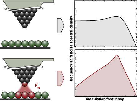
Noise in NC-AFM measurements with significant tip–sample interaction
- Jannis Lübbe,
- Matthias Temmen,
- Philipp Rahe and
- Michael Reichling
Beilstein J. Nanotechnol. 2016, 7, 1885–1904, doi:10.3762/bjnano.7.181


![[Graphic 32]](/bjnano/content/inline/2190-4286-7-181-i73.png?max-width=637&scale=1.18182) wit...
wit...

![[Graphic 34]](/bjnano/content/inline/2190-4286-7-181-i75.png?max-width=637&scale=1.18182) wit...
wit...


Understanding interferometry for micro-cantilever displacement detection
- Alexander von Schmidsfeld,
- Tobias Nörenberg,
- Matthias Temmen and
- Michael Reichling
Beilstein J. Nanotechnol. 2016, 7, 841–851, doi:10.3762/bjnano.7.76


![[Graphic 27]](/bjnano/content/inline/2190-4286-7-76-i36.png?max-width=637&scale=1.18182) of the noise floor of the interferometer signal as a function of the...
of the noise floor of the interferometer signal as a function of the...
Determining cantilever stiffness from thermal noise
- Jannis Lübbe,
- Matthias Temmen,
- Philipp Rahe,
- Angelika Kühnle and
- Michael Reichling
Beilstein J. Nanotechnol. 2013, 4, 227–233, doi:10.3762/bjnano.4.23


![[Graphic 34]](/bjnano/content/inline/2190-4286-4-23-i40.png?max-width=637&scale=1.18182) measured for the fundamental mode of cantilever V 4. Measureme...
measured for the fundamental mode of cantilever V 4. Measureme...


![[Graphic 23]](/bjnano/content/inline/2190-4286-4-23-i29.png?max-width=637&scale=1.18182) measured for cantilever V 4 (A0 = 16.8 nm, demodulator band...
measured for cantilever V 4 (A0 = 16.8 nm, demodulator band...
Thermal noise limit for ultra-high vacuum noncontact atomic force microscopy
- Jannis Lübbe,
- Matthias Temmen,
- Sebastian Rode,
- Philipp Rahe,
- Angelika Kühnle and
- Michael Reichling
Beilstein J. Nanotechnol. 2013, 4, 32–44, doi:10.3762/bjnano.4.4


![[Graphic 53]](/bjnano/content/inline/2190-4286-4-4-i64.png?max-width=637&scale=1.18182) =
= ![[Graphic 32]](/bjnano/content/inline/2190-4286-4-4-i43.png?max-width=637&scale=1.18182) f...
f...


![[Graphic 56]](/bjnano/content/inline/2190-4286-4-4-i67.png?max-width=637&scale=1.18182) using three diff...
using three diff...

Dimer/tetramer motifs determine amphiphilic hydrazine fibril structures on graphite
- Loji K. Thomas,
- Nadine Diek,
- Uwe Beginn and
- Michael Reichling
Beilstein J. Nanotechnol. 2012, 3, 658–666, doi:10.3762/bjnano.3.75


