


Abstract
Using the mumax3 program, we have shown that the interparticle dipole interaction affects the shape of hysteresis loops in stationary clusters of single-domain iron nanoparticles. We have determined how the magnetic state of nanoparticles changes depending on the thickness of the oxide shell, the distance between the particles, and the presence of particles in the vicinity. The magnetic state of nanoparticles with multidirectional magnetic crystalline anisotropy axes has been calculated at the external magnetic field and dipole fields of neighboring particles.
Introduction
Magnetic nanoparticles are widely studied for various applications, for example, in medicine [1-3] and electronics [4-6]; in particular, they have been studied quite extensively by theoretical methods [7]. Nowadays, the question of transitions to a single-domain and superparamagnetic state for various ferromagnetic metals and alloys is still relevant when changing the size or configuration of nanostructures. An actual problem is the visualization of the magnetic configurations that appear in real samples. For this purpose, experimental magneto-optical methods are used to obtain distributions of magnetic moments and dipole fields [8].
The most frequently measured characteristics of magnetic nanoparticles are the magnetic hysteresis loops, which are influenced by shape, internal magnetic properties, and external fields. Although the Stoner–Wohlfarth model for a single magnetic particle is well known, real experiments do not investigate nanoparticles separately, but rather powders or nanocomposites. In the case of ferromagnetic nanoparticles, we can expect that a large contribution should be induced by the dipole fields of neighboring particles if the latter are located close enough. These fields should also affect the magnetic state of the particles if they are located on the boundary between the multidomain and single-domain critical sizes. Moreover, metal nanoparticles are always multilayered systems of the core–shell type, in which the surface layer can be an oxide or another chemically stable coating (carbon, SiO2, organic). The surface layers create an additional distance between the ferromagnetic cores of the particles and change the magnetic properties of each particle in the powder. A more complex case occurs when the surface layer is a ferri- or ferromagnetic oxide, as in the case of iron nanoparticles. The ordering of spins on the surface might be an additional peculiarity. These features complicate the modeling of nanoparticle powder systems, and it becomes necessary to apply numerical calculations.
In previously published articles on calculations of the mutual magnetization of nanoparticles [9,10], however, the particles were considered together using various simplifications, such as the macrospin approximation and the similar direction of the anisotropy axes, as well as particle diameters larger than the single-domain size (more than 45 nm at least). In these articles, two characteristic collective effects of mutual magnetization in a particle system on its hysteresis properties were implicitly noted, that is, compression [9-11] and inversion [12] of the hysteresis loop. Experimental studies of nanoparticles have previously shown a decrease in the coercive force with increasing particle size [13] and powder packing density.
Quantitative estimates of the distances at which particles begin to “sense” each other, field strength values, and visual information about possible structures are necessary for understanding the microscopic characteristics of magnets and are useful for interpreting experimental data on magnetization and local magnetic resonance methods. This paper presents the results of micromagnetic calculations of individual single-domain iron particles and their systems, including the diameters from 10 to 26 nm and clusters of 30 particles of different diameters arranged according to a random algorithm. Magnetic states and field configurations are modeled and analyzed in systems of ferromagnetic nanoparticles near the single-domain-to-multidomain transition, and in the single-domain state, taking into account the anisotropy axes and core–shell structure.
Methods
The simulation was performed in the mumax3 software. The simulation results were limited to a static problem without temperature taken into account, so the superparamagnetic transition was not considered. Micromagnetic modeling was carried out using the standard algorithms of the program, using Runge–Kutta minimization of the total energy included in the Landau–Lifshitz equation, which considered the Zeeman interaction with an external field, magnetostatic and exchange interactions, and anisotropy energies [14]. In the case of a static equation (dM/dt = 0), the minimum energy is determined by the zero values of the effective field (the Landau–Lifshitz equation has the form [M × Heff] = 0). At the beginning of the minimization procedure, the direction of magnetization was preset randomly for each calculation cell. For core–shell systems (regions 1 and 2, respectively, see Section “Influence of the shell on the magnetic state of iron nanoparticles”), the scaling factor of the exchange ext_ScaleExchange (1, 2, A) at the boundary between the regions was A = 0; 1 to demonstrate the role of the exchange interaction (for example, if the temperature rises).
We assumed that micromagnetic modeling is applicable for solving the problem since the sizes of the nanoparticles under study were two orders of magnitude larger than the iron crystal lattice parameter (a = 0.2866 nm and the particle diameter is about 15 nm), and the size of the computational cell (1 nm) was smaller than the characteristic length of the exchange interaction in iron 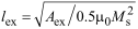 = 3.3 nm. We used the following values of, respectively, saturation magnetization, stiffness constant, and cubic anisotropy constant of iron, Ms = 1.7 × 10⁶ A/m, Aex = 2.1 × 10⁻¹¹ J/m, Kc1 = 4.8 × 10⁴ J/m3 [15], and of maghemite (γ-Fe2O3), Ms = 4 × 10⁵ A/m, Aex = 1.1 × 10⁻¹¹ J/m, Kc1 = 2.3 × 10⁴ J/m3 [16].
The calculation area for the simulation of a single particle had a size of 32 × 32 × 32 cells (nm3), the area for core–shell particles had the size 64 × 64 × 64 cells (nm3), and the calculation area for multiparticle systems was 128 × 128 × 128 cells (nm3). The boundaries of the mesh were opened. The highest smoothing was set for the nanoparticle boundaries (command EdgeSmooth = 8 divides every boundary cell into 512 subcells and rescales the saturation magnetization). The minimization parameters (including the discrepancy) had standard values for the ”relax()” procedure [14]. The fixation of spins on the surface was not predetermined for the micromagnetic calculations.
Calculations were performed using a GeForce RTX 3070 video card. Depending on the task, the calculation times were minutes (one particle) up to two weeks (nanoparticle cluster).
Results and Discussion
Calculation of the single-domain size of a nanoparticle
During the preliminary calculations using a simple search method, we obtained the single-domain limit of iron particles approximately equal to 25 nm. The magnetization was calculated in a multidomain spherical particle (26 nm) without and with an applied magnetic field (Figure 1a,b). The magnetic ordering of the particle demonstrated a curling state [17].
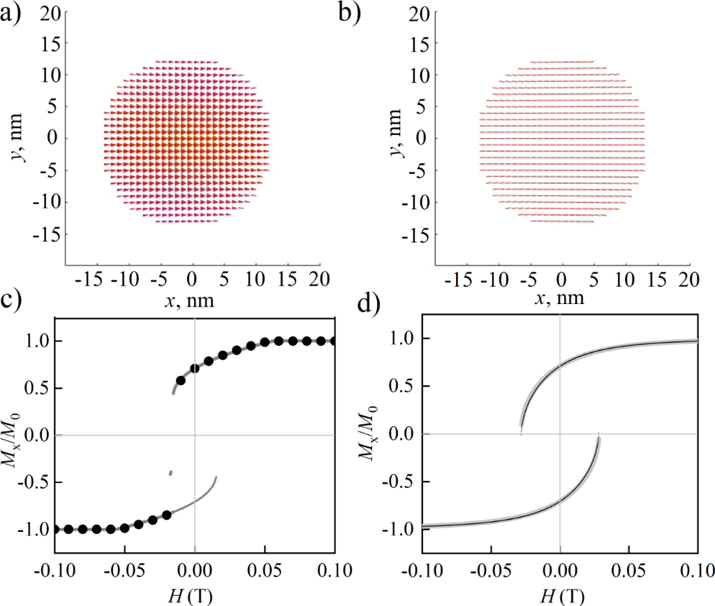
Figure 1: Magnetization of an iron nanoparticle (larger than the single-domain size, 26 nm) at the external magnetic field of 0 T (a) and 0.1 T (b). Hysteresis loops of a single-domain particle, 24 nm, obtained using the Stoner–Wohlfarth analytical model (gray line) and in mumax3 (black dots) in the field directed along the [101] direction, in the cases of cubic anisotropy along the coordinate axes (c) and uniaxial anisotropy (d) along the z-axis.
Figure 1: Magnetization of an iron nanoparticle (larger than the single-domain size, 26 nm) at the external m...
In order to verify the results of mumax3, we compared the hysteresis loops (Figure 1с,d) from numerical and analytical calculations for minimizing the total energy of a single-domain particle. The energy in the Stoner–Wohlfarth model contained the anisotropy and Zeeman contributions: for cubic anisotropy W = 0.5K(Mx2My2 + Mx2Mz2 + My2Mz2) − H·M [18], for uniaxial anisotropy W = HAMz − H·M [19]; K and HA are the anisotropy constants, M is the magnetization, and H is the magnetic field strength. The points on the hysteresis loop were normalized projections of the magnetization to the field direction. The directions of minimal energy Mmin (θmin, φmin) were determined as minima of the function of potential W for preset values and directions of anisotropy and external field strength. Further, the projection of the magnetization Mmin to the external field H was determined using the scalar product cos α = H·Mmin/|H||Mmin|. The field magnetization projection determined the points on the hysteresis loop M/M0 = cos α. This algorithm was repeated for 1000 values of the H field in the range |H| ∈ [−0.1;+0.1]. In mumax3, the dipole (Bdemag), exchange (Bexch), anisotropy (Banis), and Zeeman (Bext) interactions were taken into account: ε = −0.5M·(Bdemag + Bexch + Banis + Bext), and energy minima were calculated using the Runge–Kutta method [14].
It is clear that for a single-domain particle (as in Figure 1b), a uniform orientation of the magnetic moments at the particle boundary takes place. The opposite might be expected due to the influence of dipole magnetic fields or nanoscale boundary effects.
Influence of the shell on the magnetic state of iron nanoparticles
Iron nanoparticles in real samples can be covered with a “non-magnetic” shell, which only regulates the distances between the particles in the material. Another shell type is a ferromagnetic oxide, which causes a significant interaction between the magnetic metal core and the magnetic oxide shell. In a particle (30 nm) with a ferromagnetic iron core larger than the single-domain size, the shell orders according to the magnetostatic field of the core in the absence of an exchange interaction (ext_ScaleExchange (1,2,0)) between the iron core (27 nm) and the soft-magnetic γ-Fe2O3 (1.5 nm) shell (Figure 2a,c,e). With a shell thickness of 4.5 or 7.5 nm, core and shell order almost independently. The consideration of the exchange interaction between the particle’s core and its shell (Figure 2b,d,f) leads to the conclusion that the magnetic moments in the shell align co-directionally with those in the core, which presumably appears due to the higher value of the anisotropy constant of iron than that of γ-Fe2O3. It is notable that the curl axis in Figure 2b differs from the core anisotropy axes aligned with the coordinate axes.
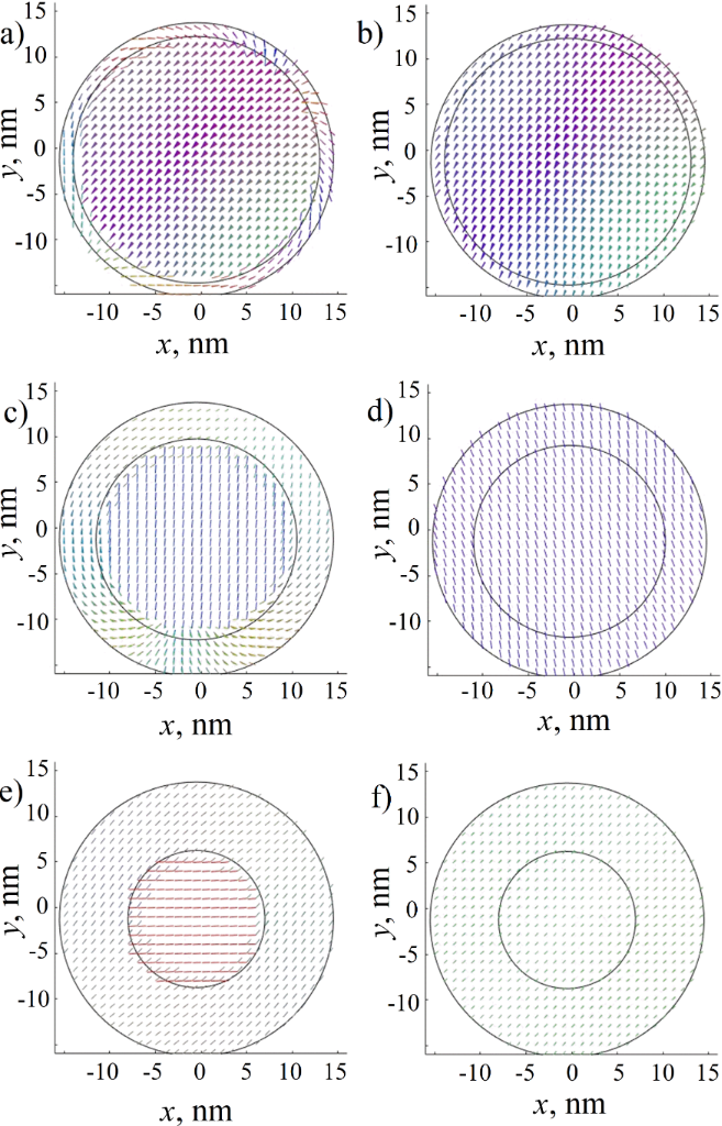
Figure 2: Magnetic moments of an iron nanoparticle with Fe2O3 maghemite shell. The cross section of the largest diameter of the calculated three-dimensional model is shown. The borders of the regions are approximately marked with black lines. (a, b) Particle with 27 nm core and 1.5 nm shell with an exchange parameter of 0 (a) and 1 (b) between regions. (c, d) Particle with 21 nm core and 4.5 nm shell with an exchange parameter of 0 (c) and 1 (d) between regions. (e, f) Particle with 15 nm core and 7.5 nm shell with an exchange parameter of 0 (e) and 1 (f) between regions.
Figure 2: Magnetic moments of an iron nanoparticle with Fe2O3 maghemite shell. The cross section of the large...
In mumax3 calculations, we considered a pure iron crystal with vanished dislocations and other defects. The obtained result represents the usual behavior of magnetic ordering in 20 nm nanoparticles (note that the single-domain diameter of iron particles equals to 25–30 nm) and contradicts the models of ultrafine nanoparticles with domain walls [20]. During calculations of the core–shell model, we chose minimum (0%) and maximum (100%) values of the exchange interaction between core and shell of the particle. The consideration of cores and shells as domains leads us to the conclusion that a magnetically soft shell of several nanometers follows the magnetic ordering of the core.
In [20], the authors suggested a model consisting of cobalt nanoparticles with a ferromagnetic core, a ferromagnetic spin-canted interface, and an antiferromagnetic oxide shell. Conclusions about the interface resulted from the observation of the NMR line similar to the signal of domain walls. The authors emphasized that a domain wall cannot exist in very small cobalt nanoparticles less than 34–56 nm, while they examined samples from 5 to 30 nm. Our calculations have shown that the exchange interaction and dipole field configuration should not allow the proposed model to be stable, taking into account that cobalt has an about ten times higher magnetic anisotropy than iron. A complex calculation of the exchange interactions between the core and shell is also presented in [21]. The authors of [20] mentioned that samples probably have a large size distribution, and the domain walls may be attributed to them. This conclusion agrees with our model rather than the previous one.
Based on the presented calculation results, we concluded that a soft magnetic shell should not significantly affect the magnetic ordering in nanoparticles, that is, the oxide shell follows the magnetic ordering of the core. In the case of a thin shell (1–3 nm), we obtained ordering along the iron anisotropy axes. Consequently, although the dipole fields become weaker with shell growth, their magnetic directions remain the same as those of pure particles. And the conclusions made for pure iron particles hold true for oxide-coated ones as well as for any similar particles at relevant distances and diameters.
The magnetic moments of core and shell can be calculated via their volumes (note that the saturation magnetizations of iron and maghemite are 17 × 105 and 4 × 10⁵ A/m, respectively). If we operate with pure iron particles of 20 nm diameter and core–shell particles of 17 nm core and 1.5 nm shell, then we obtain moments of Mpure = 7.12 × 10⁻¹⁸ A·m2, Mcore–shell = (4.37 + 0.65) × 10−18 A·m2, which are values of the same order of magnitude. Hence, we are able to model close-packed pure iron particles with higher magnetostatic fields in order to highlight characteristic effects of their dipole interactions on the magnetic hysteresis.
It is significant that we calculated pure particles at non-zero distances; however, in Figure 2e,f we show that a thick shell of 7.5 nm is able to sufficiently change the magnetic order in the particle. Moreover, for dense packaging, it is necessary to consider a more complex problem, the particles may come into contact and demonstrate sufficient exchange (“non-dipolar”) interaction with sufficient change in the magnetic state of the complex figure of agglutinated particles.
Mutual magnetization of two particles
A system of two particles is an example of a simple interparticle interaction through a magnetostatic field. We clarified whether a particle can switch between single-domain and multidomain states depending on the induced dipole fields of another particle. It was shown above that a relatively small external magnetic field can induce this transition (Figure 1). After the simulation of two particles (smaller and larger than single-domain size), we concluded that the field of a single-domain particle stabilizes a multidomain (curling) particle depending on the distance between them (Figure 3а,b). For more detailed data on the particles at distances from 1 to 17 nm, see section “Data availability”.
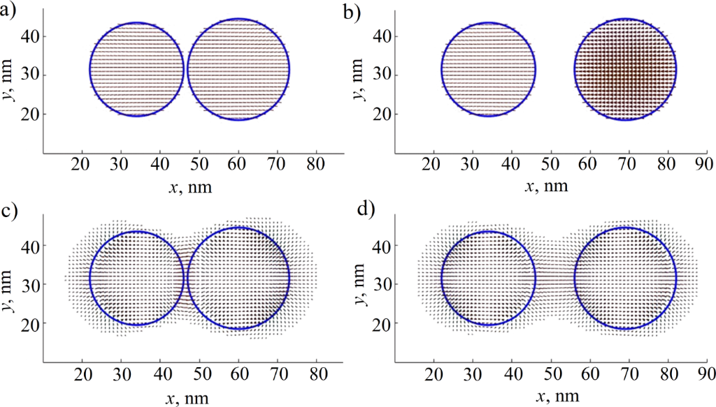
Figure 3: Magnetic moments of single-domain (24 nm) and multidomain (26 nm) particles at distances of 1 nm (a) and 10 nm (b), and the static field distribution for the same system (c, d). The cross section of the largest diameter of the calculated three-dimensional model and the magnetic field strength greater than 0.4 T are shown. Blue circles indicate the particle boundaries.
Figure 3: Magnetic moments of single-domain (24 nm) and multidomain (26 nm) particles at distances of 1 nm (a...
The point with the highest value of the magnetostatic field strength (Bdemag) lies between the particles (Figure 3c,d) and has a value of Bdemag ≈ 2.66 T at a distance of 1 nm; Bdemag ≈ 1.4 T if the distance is 10 nm. These values are of the same order as the saturation magnetization Ms of the particles (Ms ≈ 1700 kA/m of iron when the electromagnetic induction is B ≈ 2.136 T, B = μ0(H + Ms), with the first term equal to zero). This is the result of the geometrical superposition of the demagnetizing fields of the two particles. In both cases, these fields may exceed values of the saturation fields of 0.7 T for ferromagnetic single-domain iron nanopowder. The demagnetizing field created is high enough to change the magnetic state of neighboring particles.
Hysteresis loops were calculated for two single-domain iron particles with diameters of 20 nm and cubic anisotropy axes (in the directions [010], [101], and [−101]) co-directed along the line between the particle centers or perpendicular to it. It was found that their hysteresis loops (Figure 4a,b) widen compared with a single particle. It might be described as a stabilizing effect of mutually induced magnetostatic fields: The saturation for particles at a distance of 1 nm is about 1.5 times harder than for equal particles at a distance of 5 nm. The loop narrows with increasing distance between the particles (Figure 4c,d). This behavior can be explained within the framework of the Stoner–Wohlfarth model: The total energy of the system consists of dipole interaction energy, Zeeman energy, and anisotropy energy for every particle:

The calculations allow us to obtain the values of dipole–dipole energy at 1 and 5 nm distances between two 20 nm particles (or 21 and 25 nm between their centers) equal to Edip–dip = −1.06 × 10⁻¹⁸ and −6.27 × 10⁻¹⁹ J, respectively. The system approaches minimum dipole energy if the magnetizations of two particles are co-directed along the axis through their centers. The energy of a 20 nm iron particle interaction with the field of 0.1 Tesla is −7.12 × 10⁻¹⁹ J. The anisotropy energy of one particle equals to Eanis = −2.01 × 10⁻¹⁹ J. The comparison of Edip–dip and Eanis i shows that the dipole interaction exceeds the anisotropy energy at a small distance of 1 nm and introduces an additional “anisotropy-like” term into the total energy. Thus, we expect an increase in coercive field and the widening of the hysteresis loop.
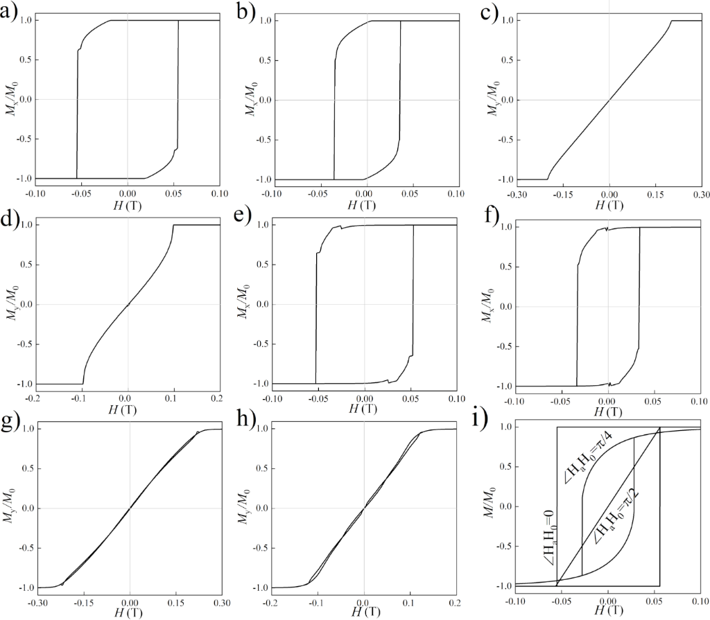
Figure 4: Hysteresis loops of longitudinal magnetization reversal of the system of two single-domain iron particles with a diameter of 20 nm with co-directed anisotropy axes at distances of 1 nm (a) and 5 nm (b); transverse magnetization reversal of the system with co-directed anisotropy axes at distances of 1 nm (c) and 5 nm (d); longitudinal magnetization reversal with multidirectional anisotropy axes at distances of 1 nm (e) and 5 nm (f); transverse magnetization reversal with multidirectional anisotropy axes at distances of 1 nm (g) and 5 nm (h). A classical example of loops of one particle with uniaxial anisotropy with three mutual orientations of the external field and anisotropy (i) is shown for comparison.
Figure 4: Hysteresis loops of longitudinal magnetization reversal of the system of two single-domain iron par...
The results of the simulation of two iron particles with different cubic anisotropy axes ([010], [101], [−101] in the first particle and [−12−1], [111], [10−1] in the second particle) qualitatively coincide with the case of equally directed anisotropy, but the loop turned out to be uneven (Figure 4e–h). This appears due to the complication of the energy landscape in the system with different anisotropy. A similar behavior has been reported in other studies [15,22]. The system exhibits multiple closely located local minima in the vicinity of the true equilibrium state. Stable states locate close to the direction of intrinsic anisotropy, and a combination of dipole fields of neighboring particles and the stepwise magnetization of the particles takes place. The steps observed in the hysteresis loops could not be connected with the field-stepping iterations in the calculations because each new calculation began with a random magnetic configuration; energy minimization for each field value was independent on the previous fields.
The comparison of hysteresis loops demonstrates that magnetostatic anisotropy plays a significant role in the system of two iron particles. This anisotropy leads to magnetization behavior that is similar to the effects of uniaxial anisotropy observed in a single particle (Figure 4i). It is possible to expect small deviations of the magnetization vectors near the surface of a single-domain particle if the particles interact. However, according to the calculations, such deviations are negligible (the magnetization projection changes by less than 1%). The same results were obtained for the subsequent calculations of the particle cluster.
Mutual magnetization in an hcp-like cluster of nanoparticles
Figure 5 shows the results of a micromagnetic calculation for an hcp-like cluster of 20 nm iron particles in order to estimate the influence of surrounding particles on the central one when they are located at a distance of 4 nm from it (Figure 5a–c). Arrows in each sphere denote the relation of the sum over the cells for the calculated magnetization in the particle to the same sum for a single “unperturbed” particle. The particle coordinates and anisotropy axes for a given configuration are presented in Supporting Information File 1, Appendix A1.

Figure 5: Magnetization and hysteresis loops of single-domain particles in a hcp-like cluster in magnetic fields of H = −0.5 T (a), 0 T (b), and +0.2 T (c). Straight orthogonal lines show the anisotropy axes. Red color indicates the predominance of the magnetization projection on the x-axis (co-directed with the external magnetic field), blue the direction along the z-axis, and green the direction along the y-axis. Hysteresis loop for the hcp-like cluster (bold line) and for the central (thin line) particle (d).
Figure 5: Magnetization and hysteresis loops of single-domain particles in a hcp-like cluster in magnetic fie...
The local hysteresis loop of the central nanoparticle (Figure 5d, thin line) has a coercive force that is an order of magnitude smaller than the value for one or a pair of particles (Figure 1, Figure 4). Single-domain particles in a cluster form a multidomain-like structure (Figure 5b) in the absence of an external field, as in bulk materials or layered structures [1,2]. The hysteresis loop demonstrates regions where the particle’s magnetization changes abruptly. We believe that it can be explained by the Barkhausen effect, or it may be related to the nonlinear dependence of the total energy of particles on the direction of magnetization. Besides this, the magnetic susceptibility changes smoothly. Such behavior may appear due to the many energetically favorable magnetostatic directions oriented toward the nearest particles.
Modeling of a nanoparticle powder: thirty randomly oriented particles of different sizes
The results most similar to real systems were obtained for a cluster of thirty nanoparticles with diameters ranging from 15 to 20 nm at distances from 3 to 5 nm among each other (Figure 6). The radii and positions of the particles were given by a random algorithm. The coordinates of the particles and the calculation parameters are given in Supporting Information File 1, Appendix A2 (for more detailed information refer to the "Data Availability Statement”).

Figure 6: Magnetization of thirty single-domain nanoparticles in magnetic fields of H = −0.5 T (a), 0 T (b), and +0.2 T (c). Total hysteresis loop for the nanoparticle’s cluster (d).
Figure 6: Magnetization of thirty single-domain nanoparticles in magnetic fields of H = −0.5 T (a), 0 T (b), ...
In the case of a complex cluster of nanoparticles, the direction of magnetization should be determined by anisotropy, static fields, and the size of the nearest particles. Relatively large particles (in the upper part of the cluster) are oriented along their anisotropy axes (Figure 6b); whereas relatively small particles are affected by the fields of larger neighbors. In a zero external field, the particles in the system form a multidomain-like structure. The cluster of single-domain particles differs from a bulk multidomain ferromagnet only by the fixed size of its “domains”, which cannot exceed the size of nanoparticles. The small value of the coercive force is typical for real nanopowders (less than 100 Oe, Figure 6d).
In [9,10], the anisotropy axes of ferromagnetic particles are oriented along the same direction. Comparing the results, we may conclude that the magnetization reversal curve of an iron nanopowder is mainly determined by the relative position of the particles and the magnetic properties of the material; this curve weakly depends on deviations from the spherical shape of the particles or the presence of an oxide shell. This may be caused by the low value of anisotropy energy in the cubic iron lattice compared to the energy of the dipole interaction.
Conclusion
Using micromagnetic calculations, we consistently demonstrated the change in the magnetic state of a nanoparticle, taking into account the shells and neighboring particles at different distances, the stabilization of the nanoparticle state in the magnetostatic field of a single neighboring particle, and the decrease in the coercive force in clusters of nanoparticles.
Based on the results of particle-in-shell modeling, it was found that a thin (approximately one tenth of the particle’s diameter) ferromagnetic shell of iron oxide does not play a significant role in the formation of the magnetic structure of a nanoparticle. A vortex nanoparticle can change its state to a single-domain state depending on its neighboring particles. The calculated deviations of magnetic moments near the surface of single-domain particles were negligible.
The stabilizing effect of the mutual magnetization of two nanoparticles with both the same and different directions of their cubic anisotropy axes was shown. Multiparticle clusters demonstrate a sharper decrease in their coercive force and a smoother movement toward saturation compared with two-particle systems and single-domain particles. Note that these effects occur in the hcp-like particle cluster and the powder cluster even when the effect of superparamagnetism is not taken into account.
Limitations
The calculations ignore the temperature and dynamics of magnetization; therefore, the possible superparamagnetic behavior of particles was not observed. This approximation is adequate for low and room temperatures since the size of the calculated particles is more than 10 nm. The use of cubic calculation cells of the mumax3 program together with the smoothing function may introduce inaccuracies in calculations at the boundaries of spherical particles (the example of non-cubic cells is presented in [23]). The fixed position of the particles limits the change in geometry, which is expectable for a real powder as a result of the particle interactions.
Supporting Information
Supporting Information features radii, positions, and anisotropy of atoms in the simulated clusters.
| Supporting Information File 1: Additional computational data. | ||
| Format: PDF | Size: 171.8 KB | Download |
Acknowledgements
The work was carried out within the framework of the state assignment of the Ministry of Science and Higher Education of the Russian Federation for the IMP UB RAS. Authors are grateful to V. D. Bessonov, V. S. Teplov, and M. A. Uimin for helpful discussions.
Funding
The calculations were made with the financial support of Russian Science Foundation (grant # 21-72-00007) https://rscf.ru/project/21-72-00007/. The work was carried out within the framework of the state assignment of the Ministry of Science and Higher Education of the Russian Federation for the IMP UB RAS theme “Function” no. 122021000035-6.
Data Availability Statement
More visual data on the magnetization reversal of nanoparticle clusters are available at the link: Germov, Alexander; Savchenko, Sergey (2025), “Micromagnetic modeling of the interaction of single-domain ferromagnetic particles in a nanopowder”, Mendeley Data, V1, https://doi.org/10.17632/r8jzxzt28s.1
References
-
Barbucci, R.; Pasqui, D.; Giani, G.; De Cagna, M.; Fini, M.; Giardino, R.; Atrei, A. Soft Matter 2011, 7, 5558–5565. doi:10.1039/c1sm05174a
Return to citation in text: [1] [2] -
Slimani, Y.; Unal, B.; Almessiere, M. A.; Hannachi, E.; Yasin, G.; Baykal, A.; Ercan, I. J. Mater. Sci.: Mater. Electron. 2020, 31, 7786–7797. doi:10.1007/s10854-020-03317-7
Return to citation in text: [1] [2] -
Abu-Bakr, A. F.; Zubarev, A. Y. Eur. Phys. J.: Spec. Top. 2020, 229, 323–329. doi:10.1140/epjst/e2019-900027-6
Return to citation in text: [1] -
Reiss, G.; Hütten, A. Nat. Mater. 2005, 4, 725–726. doi:10.1038/nmat1494
Return to citation in text: [1] -
Gliga, S.; Yan, M.; Hertel, R.; Schneider, C. M. Phys. Rev. B 2008, 77, 060404(R). doi:10.1103/physrevb.77.060404
Return to citation in text: [1] -
Poornaprakash, B.; Ramu, S.; Subramanyam, K.; Kim, Y. L.; Kumar, M.; Pratap Reddy, M. S. Ceram. Int. 2021, 47, 18557–18564. doi:10.1016/j.ceramint.2021.03.181
Return to citation in text: [1] -
Nikiforov, V. N.; Ignatenko, A. N.; Irkhin, V. Y. J. Exp. Theor. Phys. 2017, 124, 304–310. doi:10.1134/s1063776117010046
Return to citation in text: [1] -
Ivanov, V. E.; Boguslavskiy, L. G.; Feshchenko, A. A.; Andreev, S. V.; Lepalovskij, V. N. J. Magn. Magn. Mater. 2024, 590, 171681. doi:10.1016/j.jmmm.2023.171681
Return to citation in text: [1] -
Blachowicz, T.; Grzybowski, J.; Ehrmann, A. Macromol. Symp. 2022, 402, 2100381. doi:10.1002/masy.202100381
Return to citation in text: [1] [2] [3] -
Behbahani, R.; Plumer, M. L.; Saika-Voivod, I. Phys. Rev. Appl. 2022, 18, 034034. doi:10.1103/physrevapplied.18.034034
Return to citation in text: [1] [2] [3] -
Redžić, D. V. J. Phys. D: Appl. Phys. 2006, 39, 4136–4141. doi:10.1088/0022-3727/39/19/003
Return to citation in text: [1] -
Takanashi, K.; Kurokawa, H.; Fujimori, H. Appl. Phys. Lett. 1993, 63, 1585–1587. doi:10.1063/1.110756
Return to citation in text: [1] -
Sivaranjani, K. S.; Antilen Jacob, G.; Justin Joseyphus, R. J. Magn. Magn. Mater. 2020, 513, 167228. doi:10.1016/j.jmmm.2020.167228
Return to citation in text: [1] -
Vansteenkiste, A.; Leliaert, J.; Dvornik, M.; Helsen, M.; Garcia-Sanchez, F.; Van Waeyenberge, B. AIP Adv. 2014, 4, 107133. doi:10.1063/1.4899186
Return to citation in text: [1] [2] [3] -
Sudsom, D.; Ehrmann, A. Nanomaterials 2021, 11, 349. doi:10.3390/nano11020349
Return to citation in text: [1] [2] -
Niraula, G.; Coaquira, J. A. H.; Zoppellaro, G.; Villar, B. M. G.; Garcia, F.; Bakuzis, A. F.; Longo, J. P. F.; Rodrigues, M. C.; Muraca, D.; Ayesh, A. I.; Sinfrônio, F. S. M.; de Menezes, A. S.; Goya, G. F.; Sharma, S. K. ACS Appl. Nano Mater. 2021, 4, 3148–3158. doi:10.1021/acsanm.1c00311
Return to citation in text: [1] -
Skomski, R.; Liu, J. P.; Sellmyer, D. J. Phys. Rev. B 1999, 60, 7359–7365. doi:10.1103/physrevb.60.7359
Return to citation in text: [1] -
Geshev, J.; Pereira, L. G.; Schmidt, J. E.; Mikhov, M. J. Appl. Phys. 2001, 90, 6243–6250. doi:10.1063/1.1415062
Return to citation in text: [1] -
Stoner, E. C.; Wohlfarth, E. P. Philos. Trans. R. Soc., A 1948, 240, 599–642. doi:10.1098/rsta.1948.0007
Return to citation in text: [1] -
Shmyreva, A. A.; Kirillov, V. E.; Dzhangurazov, E. B.; Yurkov, G. Y. Russ. J. Phys. Chem. B 2023, 17, 764–773. doi:10.1134/s1990793123030120
Return to citation in text: [1] [2] [3] -
Kapranova, K. A.; Razlivina, J.; Dmitrenko, A.; Kladko, D. V.; Vinogradov, V. V. J. Phys. Chem. C 2025, 129, 1506–1515. doi:10.1021/acs.jpcc.4c07028
Return to citation in text: [1] -
Ummelen, F. C.; Fernández-Pacheco, A.; Mansell, R.; Petit, D.; Swagten, H. J. M.; Cowburn, R. P. Appl. Phys. Lett. 2017, 110, 102405. doi:10.1063/1.4978430
Return to citation in text: [1] -
Chichay, K. A.; Lobanov, I. S.; Uzdin, V. M. Nanosyst.: Phys., Chem., Math. 2024, 15, 55–59. doi:10.17586/2220-8054-2024-15-1-55-59
Return to citation in text: [1]
| 21. | Kapranova, K. A.; Razlivina, J.; Dmitrenko, A.; Kladko, D. V.; Vinogradov, V. V. J. Phys. Chem. C 2025, 129, 1506–1515. doi:10.1021/acs.jpcc.4c07028 |
| 20. | Shmyreva, A. A.; Kirillov, V. E.; Dzhangurazov, E. B.; Yurkov, G. Y. Russ. J. Phys. Chem. B 2023, 17, 764–773. doi:10.1134/s1990793123030120 |
| 20. | Shmyreva, A. A.; Kirillov, V. E.; Dzhangurazov, E. B.; Yurkov, G. Y. Russ. J. Phys. Chem. B 2023, 17, 764–773. doi:10.1134/s1990793123030120 |
| 1. | Barbucci, R.; Pasqui, D.; Giani, G.; De Cagna, M.; Fini, M.; Giardino, R.; Atrei, A. Soft Matter 2011, 7, 5558–5565. doi:10.1039/c1sm05174a |
| 2. | Slimani, Y.; Unal, B.; Almessiere, M. A.; Hannachi, E.; Yasin, G.; Baykal, A.; Ercan, I. J. Mater. Sci.: Mater. Electron. 2020, 31, 7786–7797. doi:10.1007/s10854-020-03317-7 |
| 3. | Abu-Bakr, A. F.; Zubarev, A. Y. Eur. Phys. J.: Spec. Top. 2020, 229, 323–329. doi:10.1140/epjst/e2019-900027-6 |
| 9. | Blachowicz, T.; Grzybowski, J.; Ehrmann, A. Macromol. Symp. 2022, 402, 2100381. doi:10.1002/masy.202100381 |
| 10. | Behbahani, R.; Plumer, M. L.; Saika-Voivod, I. Phys. Rev. Appl. 2022, 18, 034034. doi:10.1103/physrevapplied.18.034034 |
| 19. | Stoner, E. C.; Wohlfarth, E. P. Philos. Trans. R. Soc., A 1948, 240, 599–642. doi:10.1098/rsta.1948.0007 |
| 8. | Ivanov, V. E.; Boguslavskiy, L. G.; Feshchenko, A. A.; Andreev, S. V.; Lepalovskij, V. N. J. Magn. Magn. Mater. 2024, 590, 171681. doi:10.1016/j.jmmm.2023.171681 |
| 14. | Vansteenkiste, A.; Leliaert, J.; Dvornik, M.; Helsen, M.; Garcia-Sanchez, F.; Van Waeyenberge, B. AIP Adv. 2014, 4, 107133. doi:10.1063/1.4899186 |
| 7. | Nikiforov, V. N.; Ignatenko, A. N.; Irkhin, V. Y. J. Exp. Theor. Phys. 2017, 124, 304–310. doi:10.1134/s1063776117010046 |
| 17. | Skomski, R.; Liu, J. P.; Sellmyer, D. J. Phys. Rev. B 1999, 60, 7359–7365. doi:10.1103/physrevb.60.7359 |
| 23. | Chichay, K. A.; Lobanov, I. S.; Uzdin, V. M. Nanosyst.: Phys., Chem., Math. 2024, 15, 55–59. doi:10.17586/2220-8054-2024-15-1-55-59 |
| 4. | Reiss, G.; Hütten, A. Nat. Mater. 2005, 4, 725–726. doi:10.1038/nmat1494 |
| 5. | Gliga, S.; Yan, M.; Hertel, R.; Schneider, C. M. Phys. Rev. B 2008, 77, 060404(R). doi:10.1103/physrevb.77.060404 |
| 6. | Poornaprakash, B.; Ramu, S.; Subramanyam, K.; Kim, Y. L.; Kumar, M.; Pratap Reddy, M. S. Ceram. Int. 2021, 47, 18557–18564. doi:10.1016/j.ceramint.2021.03.181 |
| 18. | Geshev, J.; Pereira, L. G.; Schmidt, J. E.; Mikhov, M. J. Appl. Phys. 2001, 90, 6243–6250. doi:10.1063/1.1415062 |
| 14. | Vansteenkiste, A.; Leliaert, J.; Dvornik, M.; Helsen, M.; Garcia-Sanchez, F.; Van Waeyenberge, B. AIP Adv. 2014, 4, 107133. doi:10.1063/1.4899186 |
| 16. | Niraula, G.; Coaquira, J. A. H.; Zoppellaro, G.; Villar, B. M. G.; Garcia, F.; Bakuzis, A. F.; Longo, J. P. F.; Rodrigues, M. C.; Muraca, D.; Ayesh, A. I.; Sinfrônio, F. S. M.; de Menezes, A. S.; Goya, G. F.; Sharma, S. K. ACS Appl. Nano Mater. 2021, 4, 3148–3158. doi:10.1021/acsanm.1c00311 |
| 1. | Barbucci, R.; Pasqui, D.; Giani, G.; De Cagna, M.; Fini, M.; Giardino, R.; Atrei, A. Soft Matter 2011, 7, 5558–5565. doi:10.1039/c1sm05174a |
| 2. | Slimani, Y.; Unal, B.; Almessiere, M. A.; Hannachi, E.; Yasin, G.; Baykal, A.; Ercan, I. J. Mater. Sci.: Mater. Electron. 2020, 31, 7786–7797. doi:10.1007/s10854-020-03317-7 |
| 13. | Sivaranjani, K. S.; Antilen Jacob, G.; Justin Joseyphus, R. J. Magn. Magn. Mater. 2020, 513, 167228. doi:10.1016/j.jmmm.2020.167228 |
| 14. | Vansteenkiste, A.; Leliaert, J.; Dvornik, M.; Helsen, M.; Garcia-Sanchez, F.; Van Waeyenberge, B. AIP Adv. 2014, 4, 107133. doi:10.1063/1.4899186 |
| 9. | Blachowicz, T.; Grzybowski, J.; Ehrmann, A. Macromol. Symp. 2022, 402, 2100381. doi:10.1002/masy.202100381 |
| 10. | Behbahani, R.; Plumer, M. L.; Saika-Voivod, I. Phys. Rev. Appl. 2022, 18, 034034. doi:10.1103/physrevapplied.18.034034 |
| 12. | Takanashi, K.; Kurokawa, H.; Fujimori, H. Appl. Phys. Lett. 1993, 63, 1585–1587. doi:10.1063/1.110756 |
| 20. | Shmyreva, A. A.; Kirillov, V. E.; Dzhangurazov, E. B.; Yurkov, G. Y. Russ. J. Phys. Chem. B 2023, 17, 764–773. doi:10.1134/s1990793123030120 |
| 9. | Blachowicz, T.; Grzybowski, J.; Ehrmann, A. Macromol. Symp. 2022, 402, 2100381. doi:10.1002/masy.202100381 |
| 10. | Behbahani, R.; Plumer, M. L.; Saika-Voivod, I. Phys. Rev. Appl. 2022, 18, 034034. doi:10.1103/physrevapplied.18.034034 |
| 11. | Redžić, D. V. J. Phys. D: Appl. Phys. 2006, 39, 4136–4141. doi:10.1088/0022-3727/39/19/003 |
| 15. | Sudsom, D.; Ehrmann, A. Nanomaterials 2021, 11, 349. doi:10.3390/nano11020349 |
| 15. | Sudsom, D.; Ehrmann, A. Nanomaterials 2021, 11, 349. doi:10.3390/nano11020349 |
| 22. | Ummelen, F. C.; Fernández-Pacheco, A.; Mansell, R.; Petit, D.; Swagten, H. J. M.; Cowburn, R. P. Appl. Phys. Lett. 2017, 110, 102405. doi:10.1063/1.4978430 |
© 2026 Savchenko and Germov; licensee Beilstein-Institut.
This is an open access article licensed under the terms of the Beilstein-Institut Open Access License Agreement (https://www.beilstein-journals.org/bjnano/terms), which is identical to the Creative Commons Attribution 4.0 International License (https://creativecommons.org/licenses/by/4.0). The reuse of material under this license requires that the author(s), source and license are credited. Third-party material in this article could be subject to other licenses (typically indicated in the credit line), and in this case, users are required to obtain permission from the license holder to reuse the material.