Noncontact atomic force microscopy III

Prof. Udo D. Schwarz, Yale University
The method of noncontact atomic force microscopy (NC-AFM) has evolved significantly since its introduction and it is now possible to employ the technique to visualize the internal structure of individual molecules, controllably manipulate single atoms on surfaces, and measure potential energy landscapes with unprecedented resolution. Moreover, NC-AFM is not only limited to operation under ultrahigh vacuum and it can now be utilized to study the detailed structure and even the dynamic activity of biological molecules.
This Thematic Series follows the series "Noncontact atomic force microscopy" and "Noncontact atomic force microscopy II".
Noncontact atomic force microscopy III
- Mehmet Z. Baykara and
- Udo D. Schwarz
Beilstein J. Nanotechnol. 2016, 7, 946–947, doi:10.3762/bjnano.7.86

Boosting the local anodic oxidation of silicon through carbon nanofiber atomic force microscopy probes
- Gemma Rius,
- Matteo Lorenzoni,
- Soichiro Matsui,
- Masaki Tanemura and
- Francesc Perez-Murano
Beilstein J. Nanotechnol. 2015, 6, 215–222, doi:10.3762/bjnano.6.20


A scanning probe microscope for magnetoresistive cantilevers utilizing a nested scanner design for large-area scans
- Tobias Meier,
- Alexander Förste,
- Ali Tavassolizadeh,
- Karsten Rott,
- Dirk Meyners,
- Roland Gröger,
- Günter Reiss,
- Eckhard Quandt,
- Thomas Schimmel and
- Hendrik Hölscher
Beilstein J. Nanotechnol. 2015, 6, 451–461, doi:10.3762/bjnano.6.46


Improved atomic force microscopy cantilever performance by partial reflective coating
- Zeno Schumacher,
- Yoichi Miyahara,
- Laure Aeschimann and
- Peter Grütter
Beilstein J. Nanotechnol. 2015, 6, 1450–1456, doi:10.3762/bjnano.6.150


A simple and efficient quasi 3-dimensional viscoelastic model and software for simulation of tapping-mode atomic force microscopy
- Santiago D. Solares
Beilstein J. Nanotechnol. 2015, 6, 2233–2241, doi:10.3762/bjnano.6.229


Large area scanning probe microscope in ultra-high vacuum demonstrated for electrostatic force measurements on high-voltage devices
- Urs Gysin,
- Thilo Glatzel,
- Thomas Schmölzer,
- Adolf Schöner,
- Sergey Reshanov,
- Holger Bartolf and
- Ernst Meyer
Beilstein J. Nanotechnol. 2015, 6, 2485–2497, doi:10.3762/bjnano.6.258


Efficiency improvement in the cantilever photothermal excitation method using a photothermal conversion layer
- Natsumi Inada,
- Hitoshi Asakawa,
- Taiki Kobayashi and
- Takeshi Fukuma
Beilstein J. Nanotechnol. 2016, 7, 409–417, doi:10.3762/bjnano.7.36


Length-extension resonator as a force sensor for high-resolution frequency-modulation atomic force microscopy in air
- Hannes Beyer,
- Tino Wagner and
- Andreas Stemmer
Beilstein J. Nanotechnol. 2016, 7, 432–438, doi:10.3762/bjnano.7.38


Modelling of ‘sub-atomic’ contrast resulting from back-bonding on Si(111)-7×7
- Adam Sweetman,
- Samuel P. Jarvis and
- Mohammad A. Rashid
Beilstein J. Nanotechnol. 2016, 7, 937–945, doi:10.3762/bjnano.7.85


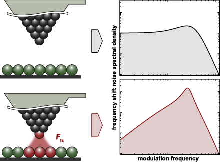
Noise in NC-AFM measurements with significant tip–sample interaction
- Jannis Lübbe,
- Matthias Temmen,
- Philipp Rahe and
- Michael Reichling
Beilstein J. Nanotechnol. 2016, 7, 1885–1904, doi:10.3762/bjnano.7.181


![[Graphic 32]](/bjnano/content/inline/2190-4286-7-181-i73.png?max-width=637&scale=1.18182) wit...
wit...

![[Graphic 34]](/bjnano/content/inline/2190-4286-7-181-i75.png?max-width=637&scale=1.18182) wit...
wit...


