Abstract
We study charge and energy transfer in two-site molecular electronic junctions in which electron transport is assisted by a vibrational mode. To understand the role of mode harmonicity/anharmonicity in transport behavior, we consider two limiting situations: (i) the mode is assumed harmonic, (ii) we truncate the mode spectrum to include only two levels, to represent an anharmonic mode. Based on the cumulant generating functions of the models, we analyze the linear-response and nonlinear performance of these junctions and demonstrate that while the electrical and thermal conductances are sensitive to whether the mode is harmonic/anharmonic, the Seebeck coefficient, the thermoelectric figure-of-merit, and the thermoelectric efficiency beyond linear response, conceal this information.
Introduction
Molecular electronic junctions offer a rich playground for exploring basic and practical questions in quantum transport, such as the interplay between electronic and nuclear dynamics in nonequilibrium situations. Theoretical and computational efforts based on minimal model Hamiltonians are largely focused on the Anderson impurity dot model which consists a single molecular electronic orbital directly coupled to biased metal leads, as well as to a particular vibrational mode [1]. Since the same molecular orbital is assumed to extend both contacts, the model allows for simulations of transport characteristics in conjugated molecular junctions with delocalized electrons.
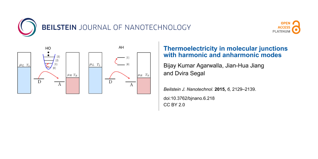
In this work, we focus on a different class of molecular junctions as depicted in Figure 1. In such systems, two electronic levels are coupled via a weak tunneling element, but electrons may effectively hop between these electronic states when interacting with a vibrational mode. This could e.g., correspond to a torsional motion bringing orthogonal π systems into an overlap as in the 2,2’-dimethylbiphenyl (DMBP) molecule recently examined in [2-4].
![[2190-4286-6-218-1]](/bjnano/content/figures/2190-4286-6-218-1.png?scale=2.0&max-width=1024&background=FFFFFF)
Figure 1: Scheme of the D–A model considered in this work. A two-site (D, A) electronic junction is coupled to either (a) a harmonic molecular mode, or (b) an anharmonic mode, represented by a two-state system. The molecular mode may further relax its energy to a phononic thermal reservoir (not depicted here), maintained at temperature Tph.
Figure 1: Scheme of the D–A model considered in this work. A two-site (D, A) electronic junction is coupled t...
This model is related to the original Aviram–Ratner construction for a donor–acceptor molecular rectifier [5]. Thus, we identify the two states here as “D” and “A”, see Figure 1, and refer to the model as the “D–A junction”. More recently, this construction was employed for exploring vibrational heating and instability under a large bias voltage [6-8]. The system is also referred to as the “dimer molecular junction” [9], or an “open spin–boson model” [10] (where the spin here represents the D and A states, the bosons correspond to the molecular vibrational modes, and the system is open, i.e., coupled to metal leads). It was utilized to study charge transfer in donor–bridge–acceptor organic molecules [11] and organic molecular semiconductors [12], as well as thermoelectric effects in quantum dot devices [13,14].
Recently, Erpenbeck et al. had provided a thorough computational study of transport characteristics with nondiagonal (or nonlocal) as well as diagonal (local) electron–vibration interactions [15]. Here, in contrast, we simplify the junction model and omit the contribution of direct tunneling between the D and A units. This simplification allows us to derive a closed (perturbative) expression for the cumulant generating function (CGF) of the model, which contains comprehensive information over transport characteristics.
Measurements of charge current and electrical conductance in single molecules hand over detailed energetic and dynamical information [16]. Complementing electrical conductance measurements, the thermopower, a linear response quantity, also referred to as the Seebeck coefficient, is utilized as an independent tool for probing the energetics of molecular junctions [17-24]. Experimental efforts identified orbital hybridization, contact-molecule energy coupling and geometry, and whether the conductance is HOMO or LUMO dominated. More generally, the thermoelectric performance beyond linear response is of interest, with the two metal leads maintained at (largely) different temperatures and chemical potentials.
What information can linear and nonlinear thermoelectric transport coefficients reveal on molecular junctions? Specifically, can they expose the underlying electron–phonon interactions and the characteristics of the vibrational modes participating in the process? Focusing on the challenge of efficient thermoelectric systems, how should we tune molecular parameters to improve heat to work conversion efficiency? These questions were examined in recent studies, a non-exhaustive list includes [13,14,25-36].
We focus here on the effect of vibrational anharmonicity on thermoelectric transport within the D–A model. To explore this issue, two limiting variants of the basic construction are examined, as displayed in Figure 1: (a) The vibration is harmonic in the so-called “harmonic oscillator” (HO) model. (b) To learn about deviations from the harmonic picture, we truncate the vibrational spectrum to include only its two lowest levels, constructing the “anharmonic” (AH) mode model. In a different context, the AH model could represent transport through molecular magnets, in which electron transfer is controlled by a spin impurity [37].
The complete information over transport behavior is contained in the respective cumulant generating functions, which we provide here for the HO and the AH models, valid under the approximation of weak electron–vibration interactions. From the CGFs, we derive expressions for charge and heat currents, and study the linear and nonlinear thermoelectric performance of the junctions. Focusing on the role of vibrational anharmonicity, we find that while it significantly influences the electrical and thermal conductances, nevertheless in the present model it does not affect heat-to-work conversion efficiency.
Model
We consider a two-site junction, where electron hopping between the D and A electronic states (creation operators ![[Graphic 1]](/bjnano/content/inline/2190-4286-6-218-i18.svg?max-width=637&scale=1.18182) and
and ![[Graphic 2]](/bjnano/content/inline/2190-4286-6-218-i19.svg?max-width=637&scale=1.18182) , respectively) is assisted by a vibrational mode. The total Hamiltonian is written as
, respectively) is assisted by a vibrational mode. The total Hamiltonian is written as
![[2190-4286-6-218-i1]](/bjnano/content/inline/2190-4286-6-218-i1.svg?max-width=590&scale=1.18182)
The molecular electronic states of energies εd,a are hybridized with their adjacent metals, collection of noninteracting electrons, by hopping elements vl and vr. Here ![[Graphic 3]](/bjnano/content/inline/2190-4286-6-218-i20.svg?max-width=637&scale=1.18182) (cj) is a fermionic creation (annihilation) operator. The electronic Hamiltonian (Equation 1, excluding Hvib+ Hel−vib) can be diagonalized and expressed in terms of new fermionic operators al and ar,
(cj) is a fermionic creation (annihilation) operator. The electronic Hamiltonian (Equation 1, excluding Hvib+ Hel−vib) can be diagonalized and expressed in terms of new fermionic operators al and ar,
![[2190-4286-6-218-i2]](/bjnano/content/inline/2190-4286-6-218-i2.svg?max-width=590&scale=1.18182)
The molecular operators can be expanded in the new basis as,
![[Graphic 4]](/bjnano/content/inline/2190-4286-6-218-i21.svg?max-width=637&scale=1.18182)
The γl,r coefficients satisfy [7]
![[Graphic 5]](/bjnano/content/inline/2190-4286-6-218-i22.svg?max-width=637&scale=1.18182)
δ is a positive infinitesimal number, introduced to maintain causuality.
The operators cl and cr can be expressed in terms of the new basis as
![[Graphic 6]](/bjnano/content/inline/2190-4286-6-218-i23.svg?max-width=637&scale=1.18182)
Similar expressions hold for the r set.
Back to Equation 1, Hvib and Hel−vib represent the Hamiltonians of the molecular vibrational mode and its coupling to electrons, respectively. We assume an “off-diagonal” interaction with electron hopping between local sites assisted by the vibrational mode. Assuming a local harmonic mode we write
![[2190-4286-6-218-i3]](/bjnano/content/inline/2190-4286-6-218-i3.svg?max-width=590&scale=1.18182)
with b0 (![[Graphic 7]](/bjnano/content/inline/2190-4286-6-218-i24.svg?max-width=637&scale=1.18182) ) as the annihilation (creation) operator for the vibrational mode of frequency ω0, g is the coupling parameter. The Hamiltonian (Equation 1) then becomes
) as the annihilation (creation) operator for the vibrational mode of frequency ω0, g is the coupling parameter. The Hamiltonian (Equation 1) then becomes
![[2190-4286-6-218-i4]](/bjnano/content/inline/2190-4286-6-218-i4.svg?max-width=590&scale=1.18182)
The second model considered here includes an anharmonic two-state mode. It is convenient to represent it with the Pauli matrices σx,y,z, and to write the total Hamiltonian for the junction as
![[2190-4286-6-218-i5]](/bjnano/content/inline/2190-4286-6-218-i5.svg?max-width=590&scale=1.18182)
The two models, Equation 4 and Equation 5, describe electron–hole pair generation/annihilation by de-excitation/excitation of an “impurity” (vibrational mode). The left and right reservoirs defining Hel in Equation 2 are characterized by a structured density of states since we had absorbed the D state in the L terminal, and similarly, the A level in the R metal. These electronic reservoirs are prepared in a thermodynamic state of temperature Tν = 1/(kBβν) and chemical potential μν, ν = L,R, set relative to the equilibrium chemical potential μF = 0. In our description we work with ![[Graphic 8]](/bjnano/content/inline/2190-4286-6-218-i25.svg?max-width=637&scale=1.18182) = 1 and e = 1. Units are revived in simulations.
= 1 and e = 1. Units are revived in simulations.
Transport
The complete information over steady-state charge and energy transport properties of molecular junctions is delivered by the so-called cumulant generating function ![[Graphic 9]](/bjnano/content/inline/2190-4286-6-218-i26.svg?max-width=637&scale=1.18182) , defined in terms of the characteristic function
, defined in terms of the characteristic function ![[Graphic 10]](/bjnano/content/inline/2190-4286-6-218-i27.svg?max-width=637&scale=1.18182) as
as
![[Graphic 11]](/bjnano/content/inline/2190-4286-6-218-i28.svg?max-width=637&scale=1.18182)
with
![[Graphic 12]](/bjnano/content/inline/2190-4286-6-218-i29.svg?max-width=637&scale=1.18182)
Here λe, λp are counting fields for energy and particles, respectively, defined for the right lead measurement, t is the final measurement time. The operators in this definition are ![[Graphic 13]](/bjnano/content/inline/2190-4286-6-218-i30.svg?max-width=637&scale=1.18182) , the number operator for the total charge in the right lead, and similarly
, the number operator for the total charge in the right lead, and similarly ![[Graphic 14]](/bjnano/content/inline/2190-4286-6-218-i31.svg?max-width=637&scale=1.18182) as the total energy in the same compartment. The superscript H identifies the Heisenberg picture, with operators evolving with respect to the full Hamiltonian. While closed results for the CGF can be derived for junctions of noninteracting particles [38], it is challenging to calculate this function analytically for models with interactions, see for example [39]. Our simplified D–A model is one of the very few many-body models that can be solved analytically.
as the total energy in the same compartment. The superscript H identifies the Heisenberg picture, with operators evolving with respect to the full Hamiltonian. While closed results for the CGF can be derived for junctions of noninteracting particles [38], it is challenging to calculate this function analytically for models with interactions, see for example [39]. Our simplified D–A model is one of the very few many-body models that can be solved analytically.
The CGF of the harmonic-mode junction (Equation 4) can be derived using the nonequilibrium Green’s function (NEGF) technique [40,41] assuming weak interaction between electrons and the particular vibration, employing the random phase approximation (RPA) [39,42]. This scheme involves a summation over a particular set (infinite) of diagrams (ring type) in the perturbative series, taking into account all electron scattering processes that are facilitated by the absorption or emission of a single quantum ω0. Physically, this summation collects not only sequential tunneling electrons, but all coordinated multi-tunneling processes, albeit with each electron interacting with the mode to the lowest order. The derivation of the CGF is nontrivial, and it is included in a separate communication [43]. Here we provide the final result
![[2190-4286-6-218-i6]](/bjnano/content/inline/2190-4286-6-218-i6.svg?max-width=590&scale=1.18182)
The CGF of the AH model (Equation 5) can be derived based on a counting-field dependent master equation approach [7,43],
![[2190-4286-6-218-i7]](/bjnano/content/inline/2190-4286-6-218-i7.svg?max-width=590&scale=1.18182)
Both expressions are correct to second-order in the electron-vibration coupling g. It is remarkable to note on the similarity of these expressions, which were derived from separate approaches. We use the short notation λ = (λp,λe), where the counting fields are defined for right-lead measurements. It can be proved that our CGFs satisfy the fluctuation symmetry [44]
![[2190-4286-6-218-i8]](/bjnano/content/inline/2190-4286-6-218-i8.svg?max-width=590&scale=1.18182)
with Δβ = βR− βL. This result is not trivial: Schemes involving truncation of interaction elements may leave out terms inconsistently with the fluctuation symmetry.
Equation 6 and Equation 7 are expressed in terms of an upward (excitation) ![[Graphic 15]](/bjnano/content/inline/2190-4286-6-218-i32.svg?max-width=637&scale=1.18182) and a downward (de-excitation)
and a downward (de-excitation) ![[Graphic 16]](/bjnano/content/inline/2190-4286-6-218-i33.svg?max-width=637&scale=1.18182) rates between vibrational states. The rates are additive in the two baths,
rates between vibrational states. The rates are additive in the two baths,
![[2190-4286-6-218-i9]](/bjnano/content/inline/2190-4286-6-218-i9.svg?max-width=590&scale=1.18182)
and obey the relation ![[Graphic 17]](/bjnano/content/inline/2190-4286-6-218-i34.svg?max-width=637&scale=1.18182) . They are given by Equation 10 [7,43].
. They are given by Equation 10 [7,43].
![[2190-4286-6-218-i10]](/bjnano/content/inline/2190-4286-6-218-i10.svg?max-width=590&scale=1.18182)
The rates kd and ku are evaluated from these expressions at λ = 0; fν(ε) = [exp(βν(ε− μν)) + 1]−1 is the Fermi–Dirac distribution function of the ν = L,R lead. The properties of the molecular junction are embedded within the spectral density functions, peaked around the molecular electronic energies εd,a with the broadening ΓL,R satisfying, e.g., ![[Graphic 18]](/bjnano/content/inline/2190-4286-6-218-i35.svg?max-width=637&scale=1.18182) ,
,
![[2190-4286-6-218-i11]](/bjnano/content/inline/2190-4286-6-218-i11.svg?max-width=590&scale=1.18182)
These expressions are reached through the diagonalization procedure of the electronic Hamiltonian while ignoring the real principal value term, responsible for a small energy shift of εd,a [7]. In what follows we take Γν as a constant independent of energy and assume broad bands with a large cutoff ±D, the largest energy scale in the problem.
We obtain currents and high order cumulants by taking derivatives of the CGF with respect to the counting fields. The particle ![[Graphic 19]](/bjnano/content/inline/2190-4286-6-218-i36.svg?max-width=637&scale=1.18182) and energy
and energy ![[Graphic 20]](/bjnano/content/inline/2190-4286-6-218-i37.svg?max-width=637&scale=1.18182) current are given by Equation 12
current are given by Equation 12
![[2190-4286-6-218-i12]](/bjnano/content/inline/2190-4286-6-218-i12.svg?max-width=590&scale=1.18182)
After some manipulations we reach the compact form for the harmonic (−) and anharmonic (+) models,
![[2190-4286-6-218-i13]](/bjnano/content/inline/2190-4286-6-218-i13.svg?max-width=590&scale=1.18182)
The rates are given by Equation 10 with λ = 0. It is notable that the only difference between the HO and AH models is the sign in the denominator. Note that we did not simplify the expression for the energy current ![[Graphic 21]](/bjnano/content/inline/2190-4286-6-218-i38.svg?max-width=637&scale=1.18182) above; the derivatives return energy transfer rates analogous to Equation 10, only with an additional energy variable in the integrand.
above; the derivatives return energy transfer rates analogous to Equation 10, only with an additional energy variable in the integrand.
While figures below only display quantities related to charge and energy currents, it is useful to emphasize that the CGF contains information on fluctuations of these currents. For example, the zero-frequency noise for charge current is given from
![[2190-4286-6-218-i14]](/bjnano/content/inline/2190-4286-6-218-i14.svg?max-width=590&scale=1.18182)
where ![[Graphic 22]](/bjnano/content/inline/2190-4286-6-218-i39.svg?max-width=637&scale=1.18182) is the second cumulant.
is the second cumulant.
Our derivation is based on the diagonal representation of the electronic Hamiltonian, thus the occupations of the molecular electronic states D and A follow the Fermi function by construction. In the weak coupling limit employed here, the back-action of the vibrational degrees of freedom on the electronic distribution is not included. While in other models [45] this back-action may be significant, here we argue that its role is rather small: Recent numerically exact path integral simulations [8] testify that this type of quantum master equation performs very well at weak to intermediate electron–vibration coupling, justifying our scheme. Note that in path integral simulations [8] the states D and A were absorbed into the metal leads as well, yet the electronic distribution was allowed to evolve in time, naturally incorporating the back-effect of vibrations on the electronic distribution in the steady-state limit.
Results
We are interested in identifying signatures of mode harmonicity in transport characteristics. We set the right contact as hot, TR > TL, and write the electronic heat current extracted from the hot bath by ![[Graphic 23]](/bjnano/content/inline/2190-4286-6-218-i40.svg?max-width=637&scale=1.18182) . The bias is applied such that μL > μR, thus the macroscopic efficiency of a thermoelectric device, converting heat to work, is given by
. The bias is applied such that μL > μR, thus the macroscopic efficiency of a thermoelectric device, converting heat to work, is given by
![[2190-4286-6-218-i15]](/bjnano/content/inline/2190-4286-6-218-i15.svg?max-width=590&scale=1.18182)
The device is operating as a thermoelectric engine when both charge and energy current flow from the hot (right) bath to the cold one. Note that according to our conventions the currents are positive when flowing from the right contact to the left.
Linear response coefficients
In linear response, i.e., close to equilibrium, the charge current ![[Graphic 24]](/bjnano/content/inline/2190-4286-6-218-i41.svg?max-width=637&scale=1.18182) and heat current
and heat current ![[Graphic 25]](/bjnano/content/inline/2190-4286-6-218-i42.svg?max-width=637&scale=1.18182) as obtained from Equation 13 can be expanded to lowest order in the bias voltage Δμ = μR− μL = eV and temperature difference ΔT = TR− TL. To re-introduce physical dimensions, we multiply the charge current by
as obtained from Equation 13 can be expanded to lowest order in the bias voltage Δμ = μR− μL = eV and temperature difference ΔT = TR− TL. To re-introduce physical dimensions, we multiply the charge current by ![[Graphic 26]](/bjnano/content/inline/2190-4286-6-218-i43.svg?max-width=637&scale=1.18182) and the heat current by
and the heat current by ![[Graphic 27]](/bjnano/content/inline/2190-4286-6-218-i44.svg?max-width=637&scale=1.18182) . The resulting expansions are cumbersome thus we write them formally in terms of the coefficients ai,j, (i,j = h,p),
. The resulting expansions are cumbersome thus we write them formally in terms of the coefficients ai,j, (i,j = h,p),
![[2190-4286-6-218-i16]](/bjnano/content/inline/2190-4286-6-218-i16.svg?max-width=590&scale=1.18182)
For ![[Graphic 28]](/bjnano/content/inline/2190-4286-6-218-i45.svg?max-width=637&scale=1.18182) and
and ![[Graphic 29]](/bjnano/content/inline/2190-4286-6-218-i46.svg?max-width=637&scale=1.18182) with Π being the Peltier coefficient [46,47], we identify the electrical conductance
with Π being the Peltier coefficient [46,47], we identify the electrical conductance
![[Graphic 30]](/bjnano/content/inline/2190-4286-6-218-i47.svg?max-width=637&scale=1.18182)
the thermopower
![[Graphic 31]](/bjnano/content/inline/2190-4286-6-218-i48.svg?max-width=637&scale=1.18182)
the electron contribution to the thermal conductance
![[Graphic 32]](/bjnano/content/inline/2190-4286-6-218-i49.svg?max-width=637&scale=1.18182)
and the (dimensionless) thermoelectric figure of merit
![[Graphic 33]](/bjnano/content/inline/2190-4286-6-218-i50.svg?max-width=637&scale=1.18182)
which determine the linear response thermoelectric efficiency. We obtain these coefficients numerically, by simulating Equation 13 under small biases.
Figure 2–Figure 4 below display the behavior of G, S, Σ and ZT at room temperature T =300 K for the harmonic and anharmonic-mode junctions. In the numerical simulations below the phononic contribution to the thermal conductance is ignored, assuming it to be small compared to its electronic counterpart. A quantitative analysis of the contribution of the phononic thermal conductance is included in the Discussion section. In addition, for simplicity, the junction is made spatially symmetric with Γ = ΓL,R and ε0 = εd,a. The currents are given by Equation 13, and we make the following observations: (i) The harmonic-mode model supports higher currents relative to the two-state case, but at low temperatures, ω0/T > > 1, when the excitation rate is negligible relative to the relaxation rate, the two models provide the same results. (ii) Since the expressions for the currents in the HO and the AH models are proportional to each other, the resulting thermopower and figure of merit are identical.
Figure 2 displays transport coefficients as a function of metal–molecule hybridization assuming a resonance situation kBT > ε0. The conductances show a turnover behavior in accord with Equation 11, growing with Γ for small values Γ < ε0, then falling down approximately as ![[Graphic 34]](/bjnano/content/inline/2190-4286-6-218-i51.svg?max-width=637&scale=1.18182) . The figure of merit shows a monotonic behavior, increasing when the broadening of levels becomes small Γ << T as we approach the so called “tight coupling” limit in which charge and heat currents are (optimally) proportional to each other.
. The figure of merit shows a monotonic behavior, increasing when the broadening of levels becomes small Γ << T as we approach the so called “tight coupling” limit in which charge and heat currents are (optimally) proportional to each other.
![[2190-4286-6-218-2]](/bjnano/content/figures/2190-4286-6-218-2.png?scale=2.0&max-width=1024&background=FFFFFF)
Figure 2: Linear response behavior of the donor–acceptor junction as a function of molecule–metal hybridization with a harmonic mode (full) and an anharmonic two-state system mode (dashed). (a) Normalized electrical conductance G/G0 with G0 = e2/h, the quantum of conductance per channel per spin. (b) Seebeck coefficient S. (c) Electronic thermal conductance Σ, and (d) the figure of merit ZT. Parameters are ε0 = 0.01, ω0 = 0.02, g = 0.01 in eV, room temperature T = 300 K. We assumed flat bands with a constant density of states.
Figure 2: Linear response behavior of the donor–acceptor junction as a function of molecule–metal hybridizati...
ZT can be significantly enhanced by tuning the molecule to an off-resonance situation, ε0 > kBT, Γ (Figure 3). We find that the electrical and thermal conductances strongly fall off with ε0, but the Seebeck coefficient displays a non-monotonic structure, with a maximum showing up off-resonance [48], resulting in a similar enhancement of ZT around ε0 = 0.2. It can be proven that the conductances are even functions in gate voltage, G(ε0) = G(−ε0), Σ(ε0) = Σ(−ε0) while S(ε0) = −S(−ε0), resulting in an even symmetry for ZT with gate voltage.
![[2190-4286-6-218-3]](/bjnano/content/figures/2190-4286-6-218-3.png?scale=2.0&max-width=1024&background=FFFFFF)
Figure 3: Linear response behavior of the donor–acceptor junction as a function of gate voltage. (a) Electrical conductance, (b) Seebeck coefficient, (c) electronic thermal conductance, and (d) figure of merit ZT. Parameters are the same as Figure 2 for Γ = 0.05 eV.
Figure 3: Linear response behavior of the donor–acceptor junction as a function of gate voltage. (a) Electric...
In Figure 4 we show transport coefficients as a function of the vibrational frequency. Parameters correspond to a resonant situation ε0/Γ = 1. Both G and Σ decay exponentially with ω0 when ω0 > kBT. However, the figure of merit only modestly increases with ω0 in the analyzed range due to the enhancement of S in this region. The values reported for ZT in Figure 4 can be increased by weakening the metal–molecule coupling energy Γ.
![[2190-4286-6-218-4]](/bjnano/content/figures/2190-4286-6-218-4.png?scale=2.0&max-width=1024&background=FFFFFF)
Figure 4: Linear response behavior of the donor–acceptor junction as a function of vibrational frequency ω0 for ε0 = 0.2 eV, Γ = 0.2 eV, g = 0.01 eV, and T = 300 K. (a) Electrical conductance, (b) Seebeck coefficient, (c) electronic thermal conductance, and (d) figure of merit ZT.
Figure 4: Linear response behavior of the donor–acceptor junction as a function of vibrational frequency ω0 f...
The maximal efficiency,
![[Graphic 35]](/bjnano/content/inline/2190-4286-6-218-i52.svg?max-width=637&scale=1.18182)
and the efficiency at maximum power [46],
![[Graphic 36]](/bjnano/content/inline/2190-4286-6-218-i53.svg?max-width=637&scale=1.18182)
are shown in Figure 5 as a function of ε0 and Γ for a fixed molecular frequency ω0 = 0.02 eV and temperature T = 300 K. Here, ηC = 1 − Tcold/Thot corresponds to the Carnot efficiency. By tuning the gate voltage and the molecule–lead hybridization we approach the bounds ηmax/ηC→ 1, η(Pmax)/ηC→ 1/2 [46]. Particularly, for Γ≈ 0.01 eV we obtain ηmax/ηC = 0.8 at the energy ε0 = 0.15.
![[2190-4286-6-218-5]](/bjnano/content/figures/2190-4286-6-218-5.png?scale=2.0&max-width=1024&background=FFFFFF)
Figure 5: Contour plot of linear response efficiencies as a function of hybridization Γ and electronic energies (or gate voltage) ε0. (a) Maximum efficiency. (b) Efficiency at maximum power. Parameters are ω0 = 0.02 eV and T = 300 K.
Figure 5: Contour plot of linear response efficiencies as a function of hybridization Γ and electronic energi...
Nonlinear performance
Nonlinear thermoelectric phenomena are anticipated to enhance thermoelectric response [49]. Elastic scattering theories of nonlinear thermoelectric transport have been developed, e.g., in [50-53], accounting for many-body effects in a phenomenological manner. Only few studies had considered this problem with explicit electron–phonon interactions, based on the Anderson–Holstein model [54] or Fermi Golden rule expressions [14].
In Figure 6 we simulate the current–voltage characteristics and the resulting efficiency of the D–A junction beyond linear response, by directly applying Equation 13. As discussed in previous investigations [6-8], the molecular junction may break down far from equilibrium due to the development of “vibrational instability”. This over-heating effect occurs when (electron-induced) vibrational excitation rates exceed relaxation rates. To cure this physical problem, we allow the particular vibrational mode of frequency ω0 to relax its excess energy to a secondary phonon bath of temperature Tph. This can be done rigorously at the level of the quantum master equations and within the NEGF technique [7,43] to yield the rates
![[Graphic 37]](/bjnano/content/inline/2190-4286-6-218-i54.svg?max-width=637&scale=1.18182)
![[Graphic 38]](/bjnano/content/inline/2190-4286-6-218-i55.svg?max-width=637&scale=1.18182)
with ![[Graphic 39]](/bjnano/content/inline/2190-4286-6-218-i56.svg?max-width=637&scale=1.18182) and a damping term Γph(ω0). Interestingly, we confirmed (not shown) that this additional energy relaxation process does not modify the thermoelectric efficiency displayed in Figure 6b.
and a damping term Γph(ω0). Interestingly, we confirmed (not shown) that this additional energy relaxation process does not modify the thermoelectric efficiency displayed in Figure 6b.
![[2190-4286-6-218-6]](/bjnano/content/figures/2190-4286-6-218-6.png?scale=2.0&max-width=1024&background=FFFFFF)
Figure 6: Transport beyond linear response. (a) current voltage characteristics for the harmonic (full) and anharmonic (dashed) mode models. (b) Heat to work conversion efficiency (Equation 15). Parameters are ω0 = 0.02, ε0 = 0.2, g = 0.01, Γ = 0.1, Γph = 0.002 in units of eV, and TL = 300 K, TR = 800 K and Tph = 300 K.
Figure 6: Transport beyond linear response. (a) current voltage characteristics for the harmonic (full) and a...
Discussion and Prospect
We focused on two-site electronic junctions in which electron transfer between sites is assisted by a particular mode, harmonic or anharmonic (two-state system). The complete information over steady state transport behavior is catered by the cumulant generating function, which we provide here for the HO and the AH mode models, valid under the approximation of weak electron–vibration interaction. We explored linear-response properties, the electrical and thermal conductances G and Σ, as well as the Seebeck coefficient S, the thermoelectric figure of merit ZT, and the resulting efficiency. We further examined current–voltage behavior and the heat-to-work conversion efficiency far-from-equilibrium. We found that G and Σ (more generally, the charge and energy currents) are sensitive to the properties of the mode, while S and ZT are insensitive to whether we work with a harmonic mode or a truncated two-state model.
Several comments are now in place:
(i) Genuine anharmonicity. We examined the role of mode anharmonicity by devising a two-state impurity model. It should be emphasized that in the context of molecules, the two-state impurity does not well represent vibrational anharmonicity at high temperatures, as many states should then contribute. Furthermore, it misses an explicit parameter tuning the potential anharmonicity. However, the AH model allows for a first indication on how deviations from harmonicity reflect in transport behavior. The HO and AH models have similar CGFs, yielding currents which are proportional, thus an identical thermoelectric efficiency. It can be readily shown that an n-state truncated HO provides a figure of merit identical to the infinite-level HO model, but it is interesting to perform more realistic calculations and consider, e.g., a morse potential to represent a physical anharmonic molecular vibration. In this case, an analytical form for the CGF is missing, but one could still derive the charge current directly from a quantum master equation formalism, to obtain the performance of the system. We expect that with a genuine anharmonic potential, S and ZT would show deviations from the harmonic limit, as different pathways for transport open up. Overall, we believe that our results here indicate on the minor role played by mode anharmonicity in determining heat-to-work conversion efficiency.
(ii) Direct tunneling. Our analysis was performed while neglecting direct electron tunneling between the D and A sites. This effect could be approximately re-instituted by assuming that coherent transport proceeds in parallel to phonon-assisted conduction, accounting for the coherent contribution using a Landauer expression, see, e.g., [3,14]. Indeed, path integral simulations indicted that in the D–A model, coherent and the incoherent contributions are approximately additive [8].
(iii) Strong electron-phonon interaction. The CGFs (Equation 6 and Equation 7) are exact to all orders in the metal–molecule hybridization but perturbative (to the lowest nontrivial order) in the electron phonon coupling g. This is evident from the structure of the rate constants in Equation 10, as electron transfer is facilitated by the absorption/emission of a single quantum ω0. In numerical simulations we typically employed g = 0.01 eV and ω0 = 0.02 eV. This value for g may seem large given the perturbative nature of our treatment requiring g/ω0 << 1. However, since in the present weak-coupling limit the current simply scales as g2, Equation 13, our simulations in this work are representative, and can be immediately translated for other values for g. It is of interest to generalize our results and study the performance of the junction with strong electron–phonon interaction, e.g., by using a polaronic transformation [55-59].
(iv) Phononic thermal conductance. We studied here electron transfer through molecular junctions, but did not discuss phonon transport characteristics across the junction, mediated by molecular vibrational modes. Consideration of the phononic thermal conductance κph is particularly important for a reliable estimate of ZT, as the thermal conductance Σ should include contributions from both electrons and phonons. We now estimate κph. The quantum of thermal conductance, an upper bound for ballistic conduction, is given by ![[Graphic 40]](/bjnano/content/inline/2190-4286-6-218-i57.svg?max-width=637&scale=1.18182) [60]. At room temperature, this yields κQ = 0.28 nW/K, which exceeds the electronic thermal conductance obtained in our simulations, to dominate the total thermal conductance and predict (significantly) lower values for the figure of merit. However, one should recognize that at high temperatures the ballistic bound for phonon thermal conductance is far from being saturated as was recently demonstrated in [61]. In particular, the phononic thermal conductance of a two-level junction was evaluated exactly in [62], and it significantly falls below the harmonic bound [61].
[60]. At room temperature, this yields κQ = 0.28 nW/K, which exceeds the electronic thermal conductance obtained in our simulations, to dominate the total thermal conductance and predict (significantly) lower values for the figure of merit. However, one should recognize that at high temperatures the ballistic bound for phonon thermal conductance is far from being saturated as was recently demonstrated in [61]. In particular, the phononic thermal conductance of a two-level junction was evaluated exactly in [62], and it significantly falls below the harmonic bound [61].
For a concrete estimate, we adopt the perturbative (weak mode-thermal bath) expression for the phononic current through a two-state junction developed in [63] and further examined in [64],
![[2190-4286-6-218-i17]](/bjnano/content/inline/2190-4286-6-218-i17.svg?max-width=590&scale=1.18182)
Here, gph is the interaction strength of the local vibrational mode to the phononic environments at the two terminals (assuming identical interaction strengths). The baths are characterized by their Bose–Einstein distribution functions nν(ω). In the case of a local harmonic mode, Equation 17 holds, only missing its denominator. Using ω0 = 0.02 eV, we receive an estimate for the phononic thermal conductance ![[Graphic 41]](/bjnano/content/inline/2190-4286-6-218-i58.svg?max-width=637&scale=1.18182) ,
, ![[Graphic 42]](/bjnano/content/inline/2190-4286-6-218-i59.svg?max-width=637&scale=1.18182) . Thus, as long as the mode-bath coupling gph is taken as weak, for example, gph <5 meV for the data of Figure 2, the electronic contribution to the thermal conductance dominates the total thermal conductance and our simulations are intact. Similar considerations hold for harmonic-mode junctions. Proposals to reduce the coherent phononic thermal conductance by quantum interference effects [65] and through-space designs [66] could be further considered.
. Thus, as long as the mode-bath coupling gph is taken as weak, for example, gph <5 meV for the data of Figure 2, the electronic contribution to the thermal conductance dominates the total thermal conductance and our simulations are intact. Similar considerations hold for harmonic-mode junctions. Proposals to reduce the coherent phononic thermal conductance by quantum interference effects [65] and through-space designs [66] could be further considered.
(v) High order cumulants. The cumulant generating functions, Equation 6 and Equation 7, contain significant information. For example, one could examine the (zero-frequency) current noise, to find out to what extent it can reveal microscopic molecular information.
(vi) Methodology development. The cumulant generating function of the HO model was derived from an NEGF approach [43]. The corresponding function for the AH model was reached from a master equation calculation [7,43]. Both treatments are perturbative to second order in the electron–vibration interaction. We take into account all electron scattering processes that are facilitated by the absorption or emission of a single quantum ω0. It is yet surprising to note on the direct correspondence between NEGF and master equation results, as derivations proceeded on completely different lines. In particular, the NEGF approach was done at the level of the RPA approximation to guarantee the validity of the fluctuation theorem. The master equation approach has been employed before to study currents (first cumulants) in the HO model [7], showing exact agreement with NEGF expressions presented here. This agreement, as well as supporting path integral simulations [8], indicate on the accuracy and consistency of the master equation in the present model. Given its simplicity and transparency, it is of interest to extend this method and examine higher order processes in perturbation theory, to gain further insight on the role of electron–vibration interaction in molecular conduction.
(vii) Efficiency fluctuations. We focused here only on averaged-macroscopic quantities. However, in small systems fluctuations in input heat and output power are significant, resulting in “second law violations” as predicted from the fluctuation theorem [44], to, e.g., grant efficiencies exceeding the thermodynamic bound. To analyze the distribution of efficiency, the concept of “stochastic efficiency” has been recently coined and examined [67,68]. In a separate contribution [43] we extend the present analysis and describe the characteristics of the stochastic efficiency in our model, particularly, we explore signatures of mode anharmonicity in the statistics of efficiency.
(viii) Molecular calculations. It is of interest to employ our expressions and examine heat-to-work conversion efficiency in realistic molecular junctions. Our results demonstrate that the conversion efficiency can be improved by working in the off-resonant limit, Γ/ε0 << 1, as well, when tuning ε0 through a gate voltage to ε0/kBT≈ 5. In such situations, the figure of merit ZT can be made large since one can tune S to large values (though the conductances are small). This suggests that in the D–A class of molecules one should focus on enhancing the thermopower as a promising mean for making an overall improvement in efficiency.
In our ongoing work we are pursuing some of these topics. The derivation of the CGFs employed here and the behavior of efficiency fluctuations in linear response, and beyond that, are detailed in [43]. In [14] we derive thermoelectric transport coefficients for the dissipative D–A model, beyond linear response, and describe the operation of thermoelectric diodes and transistors.
References
-
Galperin, M.; Ratner, M. A.; Nitzan, A. J. Phys.: Condens. Matter 2007, 19, 103201. doi:10.1088/0953-8984/19/10/103201
Return to citation in text: [1] -
Ballmann, S.; Härtle, R.; Coto, P. B.; Elbing, M.; Mayor, M.; Bryce, M. R.; Thoss, M.; Weber, H. B. Phys. Rev. Lett. 2012, 109, 056801. doi:10.1103/PhysRevLett.109.056801
Return to citation in text: [1] -
Markussen, T.; Thygesen, K. S. Phys. Rev. B 2014, 89, 085420. doi:10.1103/PhysRevB.89.085420
Return to citation in text: [1] [2] -
Simine, L.; Chen, W. J.; Segal, D. J. Phys. Chem. C 2015, 119, 12097–12108. doi:10.1021/jp512648f
Return to citation in text: [1] -
Aviram, A.; Ratner, M. A. Chem. Phys. Lett. 1974, 29, 277–283. doi:10.1016/0009-2614(74)85031-1
Return to citation in text: [1] -
Lü, J.-T.; Hedegård, P.; Brandbyge, M. Phys. Rev. Lett. 2011, 107, 046801. doi:10.1103/PhysRevLett.107.046801
Return to citation in text: [1] [2] -
Simine, L.; Segal, D. Phys. Chem. Chem. Phys. 2012, 14, 13820–13834. doi:10.1039/c2cp40851a
Return to citation in text: [1] [2] [3] [4] [5] [6] [7] [8] [9] -
Simine, L.; Segal, D. J. Chem. Phys. 2013, 138, 214111. doi:10.1063/1.4808108
Return to citation in text: [1] [2] [3] [4] [5] [6] -
Santamore, D. H.; Lambert, N.; Nori, F. Phys. Rev. B 2013, 87, 075422. doi:10.1103/PhysRevB.87.075422
Return to citation in text: [1] -
Aguado, R.; Brandes, T. Phys. Rev. Lett. 2004, 92, 206601. doi:10.1103/PhysRevLett.92.206601
Return to citation in text: [1] -
Berlin, Y. A.; Grozema, F. C.; Siebbeles, L. D. A.; Ratner, M. A. J. Phys. Chem. C 2008, 112, 10988–11000. doi:10.1021/jp801646g
Return to citation in text: [1] -
Coropceanu, V.; Sánchez-Carrera, R. S.; Paramonov, P.; Day, G. M.; Brédas, J.-L. J. Phys. Chem. C 2009, 113, 4679–4686. doi:10.1021/jp900157p
Return to citation in text: [1] -
Jiang, J.-H.; Entin-Wohlman, O.; Imry, Y. Phys. Rev. B 2012, 85, 075412. doi:10.1103/PhysRevB.85.075412
Return to citation in text: [1] [2] -
Jiang, J.-H.; Kulkarni, M.; Segal, D.; Imry, Y. Phys. Rev. B 2015, 92, 045309. doi:10.1103/PhysRevB.92.045309
Return to citation in text: [1] [2] [3] [4] [5] -
Erpenbeck, A.; Härtle, R.; Thoss, M. Phys. Rev. B 2015, 91, 195418. doi:10.1103/PhysRevB.91.195418
Return to citation in text: [1] -
Aradhya, S. V.; Venkataraman, L. Nat. Nanotechnol. 2013, 8, 399–410. doi:10.1038/nnano.2013.91
Return to citation in text: [1] -
Reddy, P.; Jang, S.-Y.; Segalman, R. A.; Majumdar, A. Science 2007, 315, 1568–1571. doi:10.1126/science.1137149
Return to citation in text: [1] -
Malen, J. A.; Doak, P.; Baheti, K.; Tilley, T. D.; Segalman, R. A.; Majumdar, A. Nano Lett. 2009, 9, 1164–1169. doi:10.1021/nl803814f
Return to citation in text: [1] -
Tan, A.; Sadat, S.; Reddy, P. Appl. Phys. Lett. 2010, 96, 013110. doi:10.1063/1.3291521
Return to citation in text: [1] -
Tan, A.; Balachandran, J.; Sadat, S.; Gavini, V.; Dunietz, B. D.; Jang, S.-Y.; Reddy, P. J. Am. Chem. Soc. 2011, 133, 8838–8841. doi:10.1021/ja202178k
Return to citation in text: [1] -
Guo, S.; Zhou, G.; Tao, N. Nano Lett. 2013, 13, 4326–4332. doi:10.1021/nl4021073
Return to citation in text: [1] -
Baheti, K.; Malen, J. A.; Doak, P.; Reddy, P.; Jang, S.-Y.; Tilley, T. D.; Majumdar, A.; Segalman, R. A. Nano Lett. 2008, 8, 715–719. doi:10.1021/nl072738l
Return to citation in text: [1] -
Widawsky, J. R.; Chen, W.; Vázquez, H.; Kim, T.; Breslow, R.; Hybertsen, M. S.; Venkataraman, L. Nano Lett. 2013, 13, 2889–2894. doi:10.1021/nl4012276
Return to citation in text: [1] -
Kim, Y.; Jeong, W.; Kim, K.; Lee, W.; Reddy, P. Nat. Nanotechnol. 2014, 9, 881–885. doi:10.1038/nnano.2014.209
Return to citation in text: [1] -
Koch, J.; von Oppen, F.; Oreg, Y.; Sela, E. Phys. Rev. B 2004, 70, 195107. doi:10.1103/PhysRevB.70.195107
Return to citation in text: [1] -
Segal, D. Phys. Rev. B 2005, 72, 165426. doi:10.1103/PhysRevB.72.165426
Return to citation in text: [1] -
Walczak, K. Physica B 2007, 392, 173–179. doi:10.1016/j.physb.2006.11.013
Return to citation in text: [1] -
Hsu, B. C.; Liu, Y.-S.; Lin, S. H.; Chen, Y.-C. Phys. Rev. B 2011, 83, 041404. doi:10.1103/PhysRevB.83.041404
Return to citation in text: [1] -
Wang, Y.; Liu, J.; Zhou, J.; Yang, R. J. Phys. Chem. C 2013, 117, 24716–24725. doi:10.1021/jp4084019
Return to citation in text: [1] -
Perroni, C. A.; Ninno, D.; Cataudella, V. Phys. Rev. B 2014, 90, 125421. doi:10.1103/PhysRevB.90.125421
Return to citation in text: [1] -
Ren, J.; Zhu, J.-X.; Gubernatis, J. E.; Wang, C.; Li, B. Phys. Rev. B 2012, 85, 155443. doi:10.1103/PhysRevB.85.155443
Return to citation in text: [1] -
Zhou, H.; Thingna, J.; Wang, J.-S.; Li, B. Phys. Rev. B 2015, 91, 045410. doi:10.1103/PhysRevB.91.045410
Return to citation in text: [1] -
Arrachea, L.; Bode, N.; von Oppen, F. Phys. Rev. B 2014, 90, 125450. doi:10.1103/PhysRevB.90.125450
Return to citation in text: [1] -
Entin-Wohlman, O.; Imry, Y.; Aharony, A. Phys. Rev. B 2010, 82, 115314. doi:10.1103/PhysRevB.82.115314
Return to citation in text: [1] -
Entin-Wohlman, O.; Imry, Y.; Aharony, A. Phys. Rev. B 2015, 91, 054302. doi:10.1103/PhysRevB.91.054302
Return to citation in text: [1] -
Lü, J.-T.; Zhou, H.; Jiang, J.-W.; Wang, J.-S. AIP Adv. 2015, 5, 053204. doi:10.1063/1.4917017
Return to citation in text: [1] -
Thiele, S.; Balestro, F.; Ballou, R.; Klyatskaya, S.; Ruben, M.; Wernsdorfer, W. Science 2014, 344, 1135–1138. doi:10.1126/science.1249802
Return to citation in text: [1] -
Levitov, L. S.; Lee, H.; Lesovik, G. B. J. Math. Phys. (Melville, NY, U. S.) 1996, 37, 4845–4866. doi:10.1063/1.531672
Return to citation in text: [1] -
Utsumi, Y.; Entin-Wohlman, O.; Ueda, A.; Aharony, A. Phys. Rev. B 2013, 87, 115407. doi:10.1103/PhysRevB.87.115407
Return to citation in text: [1] [2] -
Wang, J.-S.; Agarwalla, B. J.; Li, H.; Thingna, J. Front. Phys. 2014, 9, 673–697. doi:10.1007/s11467-013-0340-x
Return to citation in text: [1] -
Agarwalla, B. K.; Li, B.; Wang, J.-S. Phys. Rev. E 2012, 85, 051142. doi:10.1103/PhysRevE.85.051142
Return to citation in text: [1] -
Altland, A.; Simons, D. B. Condensed Matter Field Theory, 2nd ed.; Cambridge University Press: Cambridge, United Kingdom, 2010. doi:10.1017/CBO9780511789984
Return to citation in text: [1] -
Agarwalla, B. K.; Jiang, J.-H.; Segal, D. arXiv 2015, No. 1508.02475.
Return to citation in text: [1] [2] [3] [4] [5] [6] [7] [8] -
Evans, D. J.; Searles, D. J. Adv. Phys. 2002, 51, 1529–1585. doi:10.1080/00018730210155133
Return to citation in text: [1] [2] -
Park, T.-H.; Galperin, M. Phys. Rev. B 2011, 84, 205450. doi:10.1103/PhysRevB.84.205450
Return to citation in text: [1] -
Benenti, G.; Casati, G.; Prosen, T.; Saito, K. arXiv 2013, No. 1311.4430.
Return to citation in text: [1] [2] [3] -
Onsager, L. Phys. Rev. 1931, 37, 405–426. doi:10.1103/PhysRev.37.405
Return to citation in text: [1] -
Paulsson, M.; Datta, S. Phys. Rev. B 2003, 67, 241403. doi:10.1103/PhysRevB.67.241403
Return to citation in text: [1] -
Vashaee, D.; Shakouri, A. Phys. Rev. Lett. 2004, 92, 106103. doi:10.1103/PhysRevLett.92.106103
Return to citation in text: [1] -
Meair, J.; Jacquod, P. J. Phys.: Condens. Matter 2013, 25, 082201. doi:10.1088/0953-8984/25/8/082201
Return to citation in text: [1] -
Sánchez, D.; López, R. Phys. Rev. Lett. 2013, 110, 026804. doi:10.1103/PhysRevLett.110.026804
Return to citation in text: [1] -
Svensson, S. F.; Hoffmann, E. A.; Nakpathomkun, N.; Wu, P. M.; Xu, H. Q.; Nilsson, H. A.; Sánchez, D.; Kashcheyevs, V.; Linke, H. New J. Phys. 2013, 15, 105011. doi:10.1088/1367-2630/15/10/105011
Return to citation in text: [1] -
Whitney, R. S. Phys. Rev. B 2013, 88, 064302. doi:10.1103/PhysRevB.88.064302
Return to citation in text: [1] -
Leijnse, M.; Wegewijs, M. R.; Flensberg, K. Phys. Rev. B 2010, 82, 045412. doi:10.1103/PhysRevB.82.045412
Return to citation in text: [1] -
Maier, S.; Schmidt, T. L.; Komnik, A. Phys. Rev. B 2011, 83, 085401. doi:10.1103/PhysRevB.83.085401
Return to citation in text: [1] -
Koch, J.; Semmelhack, M.; von Oppen, F.; Nitzan, A. Phys. Rev. B 2006, 73, 155306. doi:10.1103/PhysRevB.73.155306
Return to citation in text: [1] -
Härtle, R.; Thoss, M. Phys. Rev. B 2011, 83, 125419. doi:10.1103/PhysRevB.83.125419
Return to citation in text: [1] -
Schaller, G.; Krause, T.; Brandes, T.; Esposito, M. New J. Phys. 2013, 15, 033032. doi:10.1088/1367-2630/15/3/033032
Return to citation in text: [1] -
Dong, B.; Ding, G. H.; Lei, X. L. Phys. Rev. B 2013, 88, 075414. doi:10.1103/PhysRevB.88.075414
Return to citation in text: [1] -
Rego, L. G. C.; Kirczenow, G. Phys. Rev. Lett. 1998, 81, 232–235. doi:10.1103/PhysRevLett.81.232
Return to citation in text: [1] -
Taylor, E.; Segal, D. Phys. Rev. Lett. 2015, 114, 220401. doi:10.1103/PhysRevLett.114.220401
Return to citation in text: [1] [2] -
Saito, K.; Kato, T. Phys. Rev. Lett. 2013, 111, 214301. doi:10.1103/PhysRevLett.111.214301
Return to citation in text: [1] -
Segal, D.; Nitzan, A. Phys. Rev. Lett. 2005, 94, 034301. doi:10.1103/PhysRevLett.94.034301
Return to citation in text: [1] -
Boudjada, N.; Segal, D. J. Phys. Chem. A 2014, 118, 11323–11336. doi:10.1021/jp5091685
Return to citation in text: [1] -
Markussen, T. J. Chem. Phys. 2013, 139, 244101. doi:10.1063/1.4849178
Return to citation in text: [1] -
Kiršanskas, G.; Li, Q.; Flensber, K.; Solomon, G. C.; Leijnse, M. Appl. Phys. Lett. 2014, 105, 233102. doi:10.1063/1.4903340
Return to citation in text: [1] -
Verley, G.; Willaert, T.; Van den Broeck, C.; Esposito, M. Nat. Commun. 2014, 5, No. 4721. doi:10.1038/ncomms5721
Return to citation in text: [1] -
Verley, G.; Willaert, T.; Van den Broeck, C.; Esposito, M. Phys. Rev. E 2014, 90, 052145. doi:10.1103/PhysRevE.90.052145
Return to citation in text: [1]
| 46. | Benenti, G.; Casati, G.; Prosen, T.; Saito, K. arXiv 2013, No. 1311.4430. |
| 47. | Onsager, L. Phys. Rev. 1931, 37, 405–426. doi:10.1103/PhysRev.37.405 |
| 48. | Paulsson, M.; Datta, S. Phys. Rev. B 2003, 67, 241403. doi:10.1103/PhysRevB.67.241403 |
| 7. | Simine, L.; Segal, D. Phys. Chem. Chem. Phys. 2012, 14, 13820–13834. doi:10.1039/c2cp40851a |
| 43. | Agarwalla, B. K.; Jiang, J.-H.; Segal, D. arXiv 2015, No. 1508.02475. |
| 3. | Markussen, T.; Thygesen, K. S. Phys. Rev. B 2014, 89, 085420. doi:10.1103/PhysRevB.89.085420 |
| 14. | Jiang, J.-H.; Kulkarni, M.; Segal, D.; Imry, Y. Phys. Rev. B 2015, 92, 045309. doi:10.1103/PhysRevB.92.045309 |
| 14. | Jiang, J.-H.; Kulkarni, M.; Segal, D.; Imry, Y. Phys. Rev. B 2015, 92, 045309. doi:10.1103/PhysRevB.92.045309 |
| 6. | Lü, J.-T.; Hedegård, P.; Brandbyge, M. Phys. Rev. Lett. 2011, 107, 046801. doi:10.1103/PhysRevLett.107.046801 |
| 7. | Simine, L.; Segal, D. Phys. Chem. Chem. Phys. 2012, 14, 13820–13834. doi:10.1039/c2cp40851a |
| 8. | Simine, L.; Segal, D. J. Chem. Phys. 2013, 138, 214111. doi:10.1063/1.4808108 |
| 50. | Meair, J.; Jacquod, P. J. Phys.: Condens. Matter 2013, 25, 082201. doi:10.1088/0953-8984/25/8/082201 |
| 51. | Sánchez, D.; López, R. Phys. Rev. Lett. 2013, 110, 026804. doi:10.1103/PhysRevLett.110.026804 |
| 52. | Svensson, S. F.; Hoffmann, E. A.; Nakpathomkun, N.; Wu, P. M.; Xu, H. Q.; Nilsson, H. A.; Sánchez, D.; Kashcheyevs, V.; Linke, H. New J. Phys. 2013, 15, 105011. doi:10.1088/1367-2630/15/10/105011 |
| 53. | Whitney, R. S. Phys. Rev. B 2013, 88, 064302. doi:10.1103/PhysRevB.88.064302 |
| 54. | Leijnse, M.; Wegewijs, M. R.; Flensberg, K. Phys. Rev. B 2010, 82, 045412. doi:10.1103/PhysRevB.82.045412 |
| 49. | Vashaee, D.; Shakouri, A. Phys. Rev. Lett. 2004, 92, 106103. doi:10.1103/PhysRevLett.92.106103 |
| 55. | Maier, S.; Schmidt, T. L.; Komnik, A. Phys. Rev. B 2011, 83, 085401. doi:10.1103/PhysRevB.83.085401 |
| 56. | Koch, J.; Semmelhack, M.; von Oppen, F.; Nitzan, A. Phys. Rev. B 2006, 73, 155306. doi:10.1103/PhysRevB.73.155306 |
| 57. | Härtle, R.; Thoss, M. Phys. Rev. B 2011, 83, 125419. doi:10.1103/PhysRevB.83.125419 |
| 58. | Schaller, G.; Krause, T.; Brandes, T.; Esposito, M. New J. Phys. 2013, 15, 033032. doi:10.1088/1367-2630/15/3/033032 |
| 59. | Dong, B.; Ding, G. H.; Lei, X. L. Phys. Rev. B 2013, 88, 075414. doi:10.1103/PhysRevB.88.075414 |
| 60. | Rego, L. G. C.; Kirczenow, G. Phys. Rev. Lett. 1998, 81, 232–235. doi:10.1103/PhysRevLett.81.232 |
| 66. | Kiršanskas, G.; Li, Q.; Flensber, K.; Solomon, G. C.; Leijnse, M. Appl. Phys. Lett. 2014, 105, 233102. doi:10.1063/1.4903340 |
| 64. | Boudjada, N.; Segal, D. J. Phys. Chem. A 2014, 118, 11323–11336. doi:10.1021/jp5091685 |
| 61. | Taylor, E.; Segal, D. Phys. Rev. Lett. 2015, 114, 220401. doi:10.1103/PhysRevLett.114.220401 |
| 63. | Segal, D.; Nitzan, A. Phys. Rev. Lett. 2005, 94, 034301. doi:10.1103/PhysRevLett.94.034301 |
| 61. | Taylor, E.; Segal, D. Phys. Rev. Lett. 2015, 114, 220401. doi:10.1103/PhysRevLett.114.220401 |
| 62. | Saito, K.; Kato, T. Phys. Rev. Lett. 2013, 111, 214301. doi:10.1103/PhysRevLett.111.214301 |
| 7. | Simine, L.; Segal, D. Phys. Chem. Chem. Phys. 2012, 14, 13820–13834. doi:10.1039/c2cp40851a |
| 7. | Simine, L.; Segal, D. Phys. Chem. Chem. Phys. 2012, 14, 13820–13834. doi:10.1039/c2cp40851a |
| 43. | Agarwalla, B. K.; Jiang, J.-H.; Segal, D. arXiv 2015, No. 1508.02475. |
| 1. | Galperin, M.; Ratner, M. A.; Nitzan, A. J. Phys.: Condens. Matter 2007, 19, 103201. doi:10.1088/0953-8984/19/10/103201 |
| 9. | Santamore, D. H.; Lambert, N.; Nori, F. Phys. Rev. B 2013, 87, 075422. doi:10.1103/PhysRevB.87.075422 |
| 7. | Simine, L.; Segal, D. Phys. Chem. Chem. Phys. 2012, 14, 13820–13834. doi:10.1039/c2cp40851a |
| 6. | Lü, J.-T.; Hedegård, P.; Brandbyge, M. Phys. Rev. Lett. 2011, 107, 046801. doi:10.1103/PhysRevLett.107.046801 |
| 7. | Simine, L.; Segal, D. Phys. Chem. Chem. Phys. 2012, 14, 13820–13834. doi:10.1039/c2cp40851a |
| 8. | Simine, L.; Segal, D. J. Chem. Phys. 2013, 138, 214111. doi:10.1063/1.4808108 |
| 38. | Levitov, L. S.; Lee, H.; Lesovik, G. B. J. Math. Phys. (Melville, NY, U. S.) 1996, 37, 4845–4866. doi:10.1063/1.531672 |
| 5. | Aviram, A.; Ratner, M. A. Chem. Phys. Lett. 1974, 29, 277–283. doi:10.1016/0009-2614(74)85031-1 |
| 13. | Jiang, J.-H.; Entin-Wohlman, O.; Imry, Y. Phys. Rev. B 2012, 85, 075412. doi:10.1103/PhysRevB.85.075412 |
| 14. | Jiang, J.-H.; Kulkarni, M.; Segal, D.; Imry, Y. Phys. Rev. B 2015, 92, 045309. doi:10.1103/PhysRevB.92.045309 |
| 25. | Koch, J.; von Oppen, F.; Oreg, Y.; Sela, E. Phys. Rev. B 2004, 70, 195107. doi:10.1103/PhysRevB.70.195107 |
| 26. | Segal, D. Phys. Rev. B 2005, 72, 165426. doi:10.1103/PhysRevB.72.165426 |
| 27. | Walczak, K. Physica B 2007, 392, 173–179. doi:10.1016/j.physb.2006.11.013 |
| 28. | Hsu, B. C.; Liu, Y.-S.; Lin, S. H.; Chen, Y.-C. Phys. Rev. B 2011, 83, 041404. doi:10.1103/PhysRevB.83.041404 |
| 29. | Wang, Y.; Liu, J.; Zhou, J.; Yang, R. J. Phys. Chem. C 2013, 117, 24716–24725. doi:10.1021/jp4084019 |
| 30. | Perroni, C. A.; Ninno, D.; Cataudella, V. Phys. Rev. B 2014, 90, 125421. doi:10.1103/PhysRevB.90.125421 |
| 31. | Ren, J.; Zhu, J.-X.; Gubernatis, J. E.; Wang, C.; Li, B. Phys. Rev. B 2012, 85, 155443. doi:10.1103/PhysRevB.85.155443 |
| 32. | Zhou, H.; Thingna, J.; Wang, J.-S.; Li, B. Phys. Rev. B 2015, 91, 045410. doi:10.1103/PhysRevB.91.045410 |
| 33. | Arrachea, L.; Bode, N.; von Oppen, F. Phys. Rev. B 2014, 90, 125450. doi:10.1103/PhysRevB.90.125450 |
| 34. | Entin-Wohlman, O.; Imry, Y.; Aharony, A. Phys. Rev. B 2010, 82, 115314. doi:10.1103/PhysRevB.82.115314 |
| 35. | Entin-Wohlman, O.; Imry, Y.; Aharony, A. Phys. Rev. B 2015, 91, 054302. doi:10.1103/PhysRevB.91.054302 |
| 36. | Lü, J.-T.; Zhou, H.; Jiang, J.-W.; Wang, J.-S. AIP Adv. 2015, 5, 053204. doi:10.1063/1.4917017 |
| 14. | Jiang, J.-H.; Kulkarni, M.; Segal, D.; Imry, Y. Phys. Rev. B 2015, 92, 045309. doi:10.1103/PhysRevB.92.045309 |
| 2. | Ballmann, S.; Härtle, R.; Coto, P. B.; Elbing, M.; Mayor, M.; Bryce, M. R.; Thoss, M.; Weber, H. B. Phys. Rev. Lett. 2012, 109, 056801. doi:10.1103/PhysRevLett.109.056801 |
| 3. | Markussen, T.; Thygesen, K. S. Phys. Rev. B 2014, 89, 085420. doi:10.1103/PhysRevB.89.085420 |
| 4. | Simine, L.; Chen, W. J.; Segal, D. J. Phys. Chem. C 2015, 119, 12097–12108. doi:10.1021/jp512648f |
| 37. | Thiele, S.; Balestro, F.; Ballou, R.; Klyatskaya, S.; Ruben, M.; Wernsdorfer, W. Science 2014, 344, 1135–1138. doi:10.1126/science.1249802 |
| 13. | Jiang, J.-H.; Entin-Wohlman, O.; Imry, Y. Phys. Rev. B 2012, 85, 075412. doi:10.1103/PhysRevB.85.075412 |
| 14. | Jiang, J.-H.; Kulkarni, M.; Segal, D.; Imry, Y. Phys. Rev. B 2015, 92, 045309. doi:10.1103/PhysRevB.92.045309 |
| 16. | Aradhya, S. V.; Venkataraman, L. Nat. Nanotechnol. 2013, 8, 399–410. doi:10.1038/nnano.2013.91 |
| 12. | Coropceanu, V.; Sánchez-Carrera, R. S.; Paramonov, P.; Day, G. M.; Brédas, J.-L. J. Phys. Chem. C 2009, 113, 4679–4686. doi:10.1021/jp900157p |
| 17. | Reddy, P.; Jang, S.-Y.; Segalman, R. A.; Majumdar, A. Science 2007, 315, 1568–1571. doi:10.1126/science.1137149 |
| 18. | Malen, J. A.; Doak, P.; Baheti, K.; Tilley, T. D.; Segalman, R. A.; Majumdar, A. Nano Lett. 2009, 9, 1164–1169. doi:10.1021/nl803814f |
| 19. | Tan, A.; Sadat, S.; Reddy, P. Appl. Phys. Lett. 2010, 96, 013110. doi:10.1063/1.3291521 |
| 20. | Tan, A.; Balachandran, J.; Sadat, S.; Gavini, V.; Dunietz, B. D.; Jang, S.-Y.; Reddy, P. J. Am. Chem. Soc. 2011, 133, 8838–8841. doi:10.1021/ja202178k |
| 21. | Guo, S.; Zhou, G.; Tao, N. Nano Lett. 2013, 13, 4326–4332. doi:10.1021/nl4021073 |
| 22. | Baheti, K.; Malen, J. A.; Doak, P.; Reddy, P.; Jang, S.-Y.; Tilley, T. D.; Majumdar, A.; Segalman, R. A. Nano Lett. 2008, 8, 715–719. doi:10.1021/nl072738l |
| 23. | Widawsky, J. R.; Chen, W.; Vázquez, H.; Kim, T.; Breslow, R.; Hybertsen, M. S.; Venkataraman, L. Nano Lett. 2013, 13, 2889–2894. doi:10.1021/nl4012276 |
| 24. | Kim, Y.; Jeong, W.; Kim, K.; Lee, W.; Reddy, P. Nat. Nanotechnol. 2014, 9, 881–885. doi:10.1038/nnano.2014.209 |
| 11. | Berlin, Y. A.; Grozema, F. C.; Siebbeles, L. D. A.; Ratner, M. A. J. Phys. Chem. C 2008, 112, 10988–11000. doi:10.1021/jp801646g |
| 44. | Evans, D. J.; Searles, D. J. Adv. Phys. 2002, 51, 1529–1585. doi:10.1080/00018730210155133 |
| 10. | Aguado, R.; Brandes, T. Phys. Rev. Lett. 2004, 92, 206601. doi:10.1103/PhysRevLett.92.206601 |
| 15. | Erpenbeck, A.; Härtle, R.; Thoss, M. Phys. Rev. B 2015, 91, 195418. doi:10.1103/PhysRevB.91.195418 |
| 67. | Verley, G.; Willaert, T.; Van den Broeck, C.; Esposito, M. Nat. Commun. 2014, 5, No. 4721. doi:10.1038/ncomms5721 |
| 68. | Verley, G.; Willaert, T.; Van den Broeck, C.; Esposito, M. Phys. Rev. E 2014, 90, 052145. doi:10.1103/PhysRevE.90.052145 |
| 39. | Utsumi, Y.; Entin-Wohlman, O.; Ueda, A.; Aharony, A. Phys. Rev. B 2013, 87, 115407. doi:10.1103/PhysRevB.87.115407 |
| 42. | Altland, A.; Simons, D. B. Condensed Matter Field Theory, 2nd ed.; Cambridge University Press: Cambridge, United Kingdom, 2010. doi:10.1017/CBO9780511789984 |
| 39. | Utsumi, Y.; Entin-Wohlman, O.; Ueda, A.; Aharony, A. Phys. Rev. B 2013, 87, 115407. doi:10.1103/PhysRevB.87.115407 |
| 40. | Wang, J.-S.; Agarwalla, B. J.; Li, H.; Thingna, J. Front. Phys. 2014, 9, 673–697. doi:10.1007/s11467-013-0340-x |
| 41. | Agarwalla, B. K.; Li, B.; Wang, J.-S. Phys. Rev. E 2012, 85, 051142. doi:10.1103/PhysRevE.85.051142 |
| 7. | Simine, L.; Segal, D. Phys. Chem. Chem. Phys. 2012, 14, 13820–13834. doi:10.1039/c2cp40851a |
| 45. | Park, T.-H.; Galperin, M. Phys. Rev. B 2011, 84, 205450. doi:10.1103/PhysRevB.84.205450 |
| 44. | Evans, D. J.; Searles, D. J. Adv. Phys. 2002, 51, 1529–1585. doi:10.1080/00018730210155133 |
| 7. | Simine, L.; Segal, D. Phys. Chem. Chem. Phys. 2012, 14, 13820–13834. doi:10.1039/c2cp40851a |
| 43. | Agarwalla, B. K.; Jiang, J.-H.; Segal, D. arXiv 2015, No. 1508.02475. |
| 7. | Simine, L.; Segal, D. Phys. Chem. Chem. Phys. 2012, 14, 13820–13834. doi:10.1039/c2cp40851a |
| 43. | Agarwalla, B. K.; Jiang, J.-H.; Segal, D. arXiv 2015, No. 1508.02475. |
© 2015 Agarwalla et al; licensee Beilstein-Institut.
This is an Open Access article under the terms of the Creative Commons Attribution License (http://creativecommons.org/licenses/by/2.0), which permits unrestricted use, distribution, and reproduction in any medium, provided the original work is properly cited.
The license is subject to the Beilstein Journal of Nanotechnology terms and conditions: (http://www.beilstein-journals.org/bjnano)