Topographic signatures and manipulations of Fe atoms, CO molecules and NaCl islands on superconducting Pb(111)
- Carl Drechsel,
- Philipp D’Astolfo,
- Jung-Ching Liu,
- Thilo Glatzel,
- Rémy Pawlak and
- Ernst Meyer
Beilstein J. Nanotechnol. 2022, 13, 1–9, doi:10.3762/bjnano.13.1


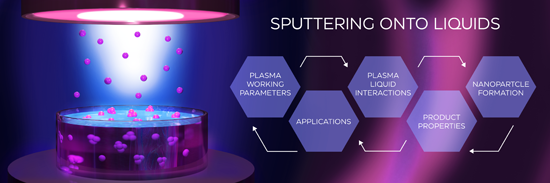
Sputtering onto liquids: a critical review
- Anastasiya Sergievskaya,
- Adrien Chauvin and
- Stephanos Konstantinidis
Beilstein J. Nanotechnol. 2022, 13, 10–53, doi:10.3762/bjnano.13.2


Effect of lubricants on the rotational transmission between solid-state gears
- Huang-Hsiang Lin,
- Jonathan Heinze,
- Alexander Croy,
- Rafael Gutiérrez and
- Gianaurelio Cuniberti
Beilstein J. Nanotechnol. 2022, 13, 54–62, doi:10.3762/bjnano.13.3


Nanoscale friction and wear of a polymer coated with graphene
- Robin Vacher and
- Astrid S. de Wijn
Beilstein J. Nanotechnol. 2022, 13, 63–73, doi:10.3762/bjnano.13.4


Influence of magnetic domain walls on all-optical magnetic toggle switching in a ferrimagnetic GdFe film
- Rahil Hosseinifar,
- Evangelos Golias,
- Ivar Kumberg,
- Quentin Guillet,
- Karl Frischmuth,
- Sangeeta Thakur,
- Mario Fix,
- Manfred Albrecht,
- Florian Kronast and
- Wolfgang Kuch
Beilstein J. Nanotechnol. 2022, 13, 74–81, doi:10.3762/bjnano.13.5


Theranostic potential of self-luminescent branched polyethyleneimine-coated superparamagnetic iron oxide nanoparticles
- Rouhollah Khodadust,
- Ozlem Unal and
- Havva Yagci Acar
Beilstein J. Nanotechnol. 2022, 13, 82–95, doi:10.3762/bjnano.13.6


Tin dioxide nanomaterial-based photocatalysts for nitrogen oxide oxidation: a review
- Viet Van Pham,
- Hong-Huy Tran,
- Thao Kim Truong and
- Thi Minh Cao
Beilstein J. Nanotechnol. 2022, 13, 96–113, doi:10.3762/bjnano.13.7


Bacterial safety study of the production process of hemoglobin-based oxygen carriers
- Axel Steffen,
- Yu Xiong,
- Radostina Georgieva,
- Ulrich Kalus and
- Hans Bäumler
Beilstein J. Nanotechnol. 2022, 13, 114–126, doi:10.3762/bjnano.13.8


A photonic crystal material for the online detection of nonpolar hydrocarbon vapors
- Evgenii S. Bolshakov,
- Aleksander V. Ivanov,
- Andrei A. Kozlov,
- Anton S. Aksenov,
- Elena V. Isanbaeva,
- Sergei E. Kushnir,
- Aleksei D. Yapryntsev,
- Aleksander E. Baranchikov and
- Yury A. Zolotov
Beilstein J. Nanotechnol. 2022, 13, 127–136, doi:10.3762/bjnano.13.9


A comprehensive review on electrospun nanohybrid membranes for wastewater treatment
- Senuri Kumarage,
- Imalka Munaweera and
- Nilwala Kottegoda
Beilstein J. Nanotechnol. 2022, 13, 137–159, doi:10.3762/bjnano.13.10


Theoretical understanding of electronic and mechanical properties of 1T′ transition metal dichalcogenide crystals
- Seyedeh Alieh Kazemi,
- Sadegh Imani Yengejeh,
- Vei Wang,
- William Wen and
- Yun Wang
Beilstein J. Nanotechnol. 2022, 13, 160–171, doi:10.3762/bjnano.13.11


Thermal oxidation process on Si(113)-(3 × 2) investigated using high-temperature scanning tunneling microscopy
- Hiroya Tanaka,
- Shinya Ohno,
- Kazushi Miki and
- Masatoshi Tanaka
Beilstein J. Nanotechnol. 2022, 13, 172–181, doi:10.3762/bjnano.13.12


Low-energy electron interaction and focused electron beam-induced deposition of molybdenum hexacarbonyl (Mo(CO)6)
- Po-Yuan Shih,
- Maicol Cipriani,
- Christian Felix Hermanns,
- Jens Oster,
- Klaus Edinger,
- Armin Gölzhäuser and
- Oddur Ingólfsson
Beilstein J. Nanotechnol. 2022, 13, 182–191, doi:10.3762/bjnano.13.13


Piezoelectric nanogenerator for bio-mechanical strain measurement
- Zafar Javed,
- Lybah Rafiq,
- Muhammad Anwaar Nazeer,
- Saqib Siddiqui,
- Muhammad Babar Ramzan,
- Muhammad Qamar Khan and
- Muhammad Salman Naeem
Beilstein J. Nanotechnol. 2022, 13, 192–200, doi:10.3762/bjnano.13.14


Engineered titania nanomaterials in advanced clinical applications
- Padmavati Sahare,
- Paulina Govea Alvarez,
- Juan Manual Sanchez Yanez,
- Gabriel Luna-Bárcenas,
- Samik Chakraborty,
- Sujay Paul and
- Miriam Estevez
Beilstein J. Nanotechnol. 2022, 13, 201–218, doi:10.3762/bjnano.13.15


Impact of device design on the electronic and optoelectronic properties of integrated Ru-terpyridine complexes
- Max Mennicken,
- Sophia Katharina Peter,
- Corinna Kaulen,
- Ulrich Simon and
- Silvia Karthäuser
Beilstein J. Nanotechnol. 2022, 13, 219–229, doi:10.3762/bjnano.13.16


Surfactant-free syntheses and pair distribution function analysis of osmium nanoparticles
- Mikkel Juelsholt,
- Jonathan Quinson,
- Emil T. S. Kjær,
- Baiyu Wang,
- Rebecca Pittkowski,
- Susan R. Cooper,
- Tiffany L. Kinnibrugh,
- Søren B. Simonsen,
- Luise Theil Kuhn,
- María Escudero-Escribano and
- Kirsten M. Ø. Jensen
Beilstein J. Nanotechnol. 2022, 13, 230–235, doi:10.3762/bjnano.13.17


Relationship between corrosion and nanoscale friction on a metallic glass
- Haoran Ma and
- Roland Bennewitz
Beilstein J. Nanotechnol. 2022, 13, 236–244, doi:10.3762/bjnano.13.18


Effects of drug concentration and PLGA addition on the properties of electrospun ampicillin trihydrate-loaded PLA nanofibers
- Tuğba Eren Böncü and
- Nurten Ozdemir
Beilstein J. Nanotechnol. 2022, 13, 245–254, doi:10.3762/bjnano.13.19


Photothermal ablation of murine melanomas by Fe3O4 nanoparticle clusters
- Xue Wang,
- Lili Xuan and
- Ying Pan
Beilstein J. Nanotechnol. 2022, 13, 255–264, doi:10.3762/bjnano.13.20


Investigation of a memory effect in a Au/(Ti–Cu)Ox-gradient thin film/TiAlV structure
- Damian Wojcieszak,
- Jarosław Domaradzki,
- Michał Mazur,
- Tomasz Kotwica and
- Danuta Kaczmarek
Beilstein J. Nanotechnol. 2022, 13, 265–273, doi:10.3762/bjnano.13.21


Systematic studies into uniform synthetic protein nanoparticles
- Nahal Habibi,
- Ava Mauser,
- Jeffery E. Raymond and
- Joerg Lahann
Beilstein J. Nanotechnol. 2022, 13, 274–283, doi:10.3762/bjnano.13.22


Coordination-assembled myricetin nanoarchitectonics for sustainably scavenging free radicals
- Xiaoyan Ma,
- Haoning Gong,
- Kenji Ogino,
- Xuehai Yan and
- Ruirui Xing
Beilstein J. Nanotechnol. 2022, 13, 284–291, doi:10.3762/bjnano.13.23


Plasma modes in capacitively coupled superconducting nanowires
- Alex Latyshev,
- Andrew G. Semenov and
- Andrei D. Zaikin
Beilstein J. Nanotechnol. 2022, 13, 292–297, doi:10.3762/bjnano.13.24


The effect of metal surface nanomorphology on the output performance of a TENG
- Yiru Wang,
- Xin Zhao,
- Yang Liu and
- Wenjun Zhou
Beilstein J. Nanotechnol. 2022, 13, 298–312, doi:10.3762/bjnano.13.25


